Gyroscope Characterization and Calibration

Test Description and Objectives

This test is designed to characterize and calibrate the ADCS gyroscopes, ensuring their precise performance under various conditions. The results will give us important information to improve the system that controls the satellite’s orientation, making the system more reliable and effective.

Test Set-Up

To conduct this test, an STM32L476RG Nucleo board is utilized as a simulator for the OBC-ADCS interface. Commands are sent to the Nucleo board, which subsequently requests data from the ADCS board.

• ADCS and Breakout board
• STM32L476RG Nucleo board
• Wires
• A computer with STM32CubeIde and Ki-Cad installed
• Calculator, pen and paper, or computer with Excel
• Protoboard
• 2 Resistances of 4.7 KOhms
• Peltier cell
• Halogen lamp
• Rotating platform with motor. In case of unavailability, use something that can produce a constant rotation.
• Power supply.

Test Plan

To calibrate the gyroscope IIM 42652 we have done the following test:

3.1 Allan's variance characterization

First, the “Random walk phenomenon” of the gyroscope has to be characterized. The method will use the Allan’s variance. Once the samples of measurements has been taken, the standard deviation of the measurements will be plotted in function of the time. The results might be similar to the following ones:

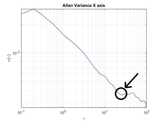
In these plots, it is observed the evolution of the standard deviation of the noise in the gyroscope samples. Approximately, in τ=10 s for the X and Z axis, and for τ=20 s, the standard variation tends to variate the slope of the line repeatedly, that happens because of the effect of the “Random walk phenomenon”.

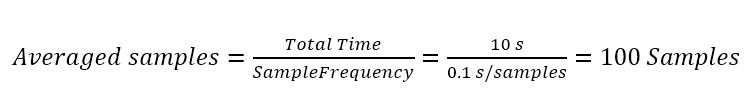
Consequently,  the gyroscope samples will be averaged for 10 seconds, using a sample frequency of 0.1 seconds. The total number samples that will be averaged is 100 samples.

The schematic used for the averaging algorithm is the following one:

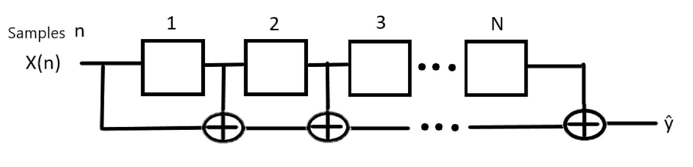
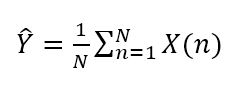
This algorithm functions as a circular queue that averages all the samples within it during each iteration, helping to reduce the effect of the "random walk phenomenon" in the gyroscope readings.

3.2 Temperature bias characterization and calibration

Afterwards, we will have to take at least 1000, or more, samples of data for each axi in differents situations using the algorithm of the previous section:

1- Static data measurements, all with a constant temperature.

• Ambient temperature, aproximately 25ºC.
• Night temperature, around 10ºC.
• Freezer temperature. around -16 ºC.
• Halogen lamp, around 40ºC.
• (optional) peltier cellwith a constant temperature different to the previous ones

2-Movement measurements

• With the rotation platform take samples of each axi in one velocity, remember to writte down the real velocity used in degrees/second and the temperature of each sample.
• With the same velocity redo the measurements now with a diferent temperature, remember to use one of the temperatures used for the previous static measurements, for example halogen lamp with 40 ºC.

After that, in order to calibrate de measurements, the following formula will be used for each axis:

                                             Data Calibrated = Data measured * sensitivity - Bias(Tº)

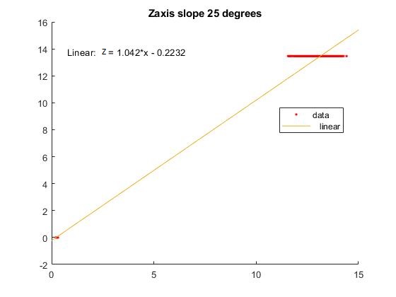
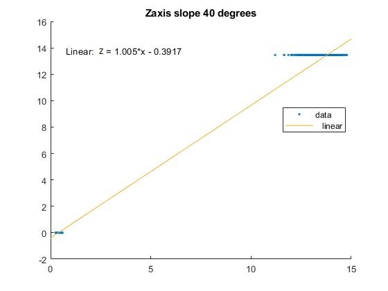
For each axis, plot the real data in function of the measured data using in the X axis the measured data and in the Y axis the real data. Afterwards, in the measured data vector use the static data and the constant velocity data, both obtained with the same temperature. Regarding the real data, also use the static real data and the real angular velocity data. Now you will have two figures, each one with different temperature, compute in both plots the line equation of the graphic and store the value of the slope coefficient of the equation.

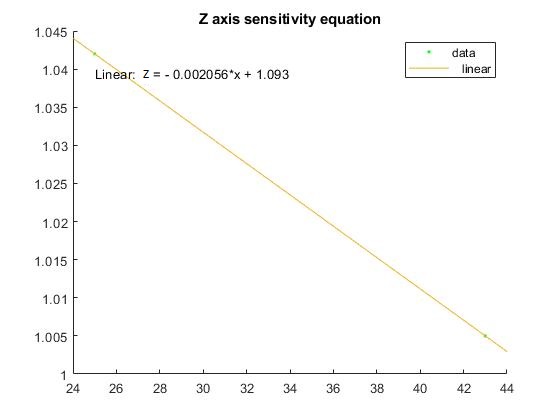
After obtaining the two slopes, one for the first temperature and the other for the second, the next step is to plot the slope, which is computed using the two previous calculated slopes, against the temperature and recalculate the line equation. This line equation will serve as the formula for calculating sensitivity as a function of temperature.

This procedure is repeated for each axis:

Axis	Slope (25 ºC)	Slope (40 ºC)	Sensitivity equation
X	1.073	1.085	Xsens=-0.0009231*T(ºC)+1.05
Y	1.026	0.9912	Ysens=-0.0029*T(ºC)+1.099
Z	1.042	1.005	Zsens=0.002056*T(ºC)+1.093

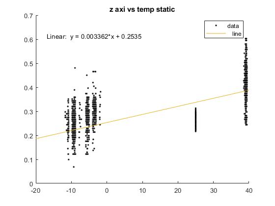
For the next step of the calibration, the measured static data versus the temperature is plotted. This graphic will show us the evolution of the bias in respect to the temperature. Then, the equation of the line will be computed, which will be used in order to compute the Bias:

            Bias( Tº) = m *  Tº(temperature) + n

The results for each axis are:

Axies	Bias equation
X	Bias=0.01388 * T(ºC)-0.1716
Y	Bias=0.0005596 * T(ºC)-0.03862
Z	Bias=0.003362 * T(ºC)+0.2535

The final calibrated data will be computed with the following equation:

Calibrated_data = Sensitivity(ºC) * Measured_data - Bias(ºC)

Test Results

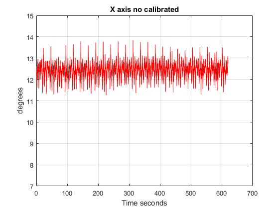
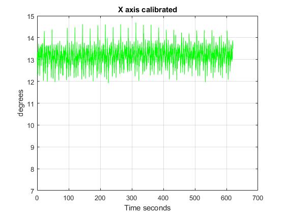
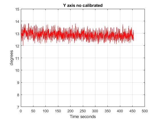
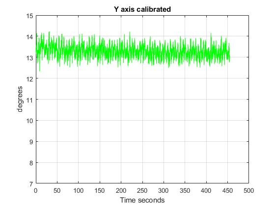
The test consisted of measurements of a real velocity of 13,6 degrees/s. The following plots show that the results of the calibration in all the axis.

                             

                             

                           

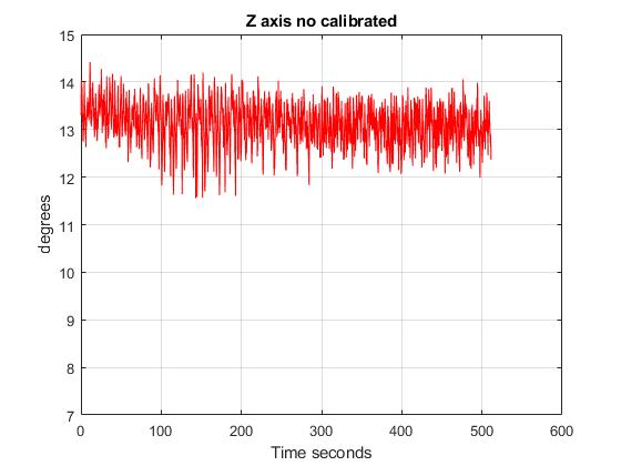
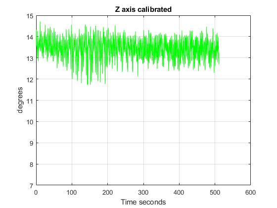
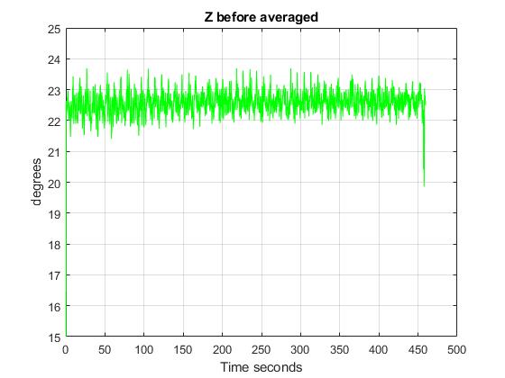
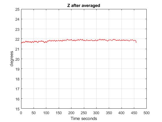
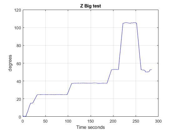
In addition, the following figures show the results of testing the averaged algorithm. The tests show how the gyroscope works once it has been calibrated. To do so, different velocities had been applied into the Z axis. Here are the results:

                       

         

Anomalies

The temperature sensor inside the IIM 42652 could work wrongly if the chip has been exposed to high temperatures during the welding process. It is recommendable to check in the IIM 42652 documentation, which is the maximum temperature that the temperature sensor can withstand without getting damaged.

Conclusions

As all the requirements has been fulfilled, the test is completed.