RFI-Dedicated Thread

RFI Thread

Introduction

Like many other subsystems, the Payload is a self-contained sub-system and so it has its own FreeRTOS Thread. This thread is concieved to be able to control each of the two RFI monitoring payloads.

As an overview, the thread is structured as secuential general operations. And each of them is a key step in the process of making the payload work.

Block Diagram

To begin, the general behavior of the code is defined, since it is basic to have it structured from the most generic functions to the most specific ones. This general structure is basic since it is the one that will be in direct ”contact” with the OBC code, and its structure and functioning requirements.

This figure, as stated above, defines how the payload code is structured and its sequential steps. Note that the discontinuous arrow indicates that once the loop has finished, the payload thread enters a sleep mode, waiting for the OBC to awaken him again to restart the loop. So, the first to take a deeper look into is going to be the Check start conditions block:

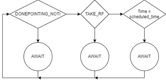
As it can be seen above, the first thing to do in order to get the payload running properly is to check if the conditions required by the Ground Station user are met, this includes three things:

The satellite is pointing at the desired region of the Earth steadily.

The order to make an RFI measurement has been truly received.

It is the scheduled moment to take the photo.

If none of these requirements are met, the thread awaits until it is signaled by the OBC and then rechecking everything again. Once the check has been succeed, it is time to Start the electronics and the timer:

Obviously, the first step is to power on the payload and consequently all its elements. Then the ADC and DAC are initialized and started. The same happens to the timer. Once they have been started it is time to make sure that they work as expected:

Now the ADC and DAC are checked and calibrated, the timer is only checked. This is done to assure that when using them in the measurements they don’t give false reading due to a malfunction. Having everything powered on, initialized and checked, the measure loop can begin:

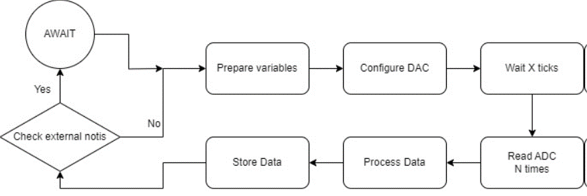
This loop is run as many times as needed in order to scan all the frequency bins forming the L or Ka bands. This scans are slow, so not to block the whole satellite system, every time a frequency bin is scanned the thread checks for notifications coming from the rest of the PQ to pause itself if necessary. Then, once the satellite does not need to have the RFI thread stop anymore, the RFI thread continues from where it was.

In order to bring the explanation to a lower level, the list below explains each block step by step:

Prepare variables: Every variable that is going to be used during the measure loop execution needs to be initialized to ensure a solid structure in the RAM (Random Access Memory).

Configure DAC: As explained in Chapter 4.2.3, the DAC (Digital to Analog Converter) is configured to make the oscillator output a certain frequency (depending on the frequency bin that wants to be analyzed) by inputting the accordingly calculated voltage.

Wait X ticks: a yet to be calculated amount of clock ticks is waited to ensure that the frequency from the CO (Controlled Oscillator) is stable.
- The amount of ticks needed depends on the clock speed, and DAC configuration and stabilisation time, which can be found in the microcontroller datasheet. The amount of ticks awaited must exceed an equivalent time of 7.5us.
- This calculation is done taking into account the clock speed and therefore the tick period. This results in the next formula: X = 7.5/fclk[MHz]

Read ADC N times: The ADC reads the voltage from the RSSI output and converts it to a digital value. This is done N times for the posterior time domain analysis of the samples. The value of N is calculated by dividing the BW (Bandwidth) of the band with the RSSI BW, resulting in the next formula: N = BW/BWRSSI .
- For the L band: Since the RSSI BW is 4 MHZ, the resulting N = 250 .
- For the Ka band: Since the RSSI BW is 16 MHZ, the resulting N = 63 .

Process Data: With the raw ADC (Analog to Digital Converter) values, calculate different statistical parameters to represent that frequency bin. Those will be stored, whereas the raw values will not.

Store Data: Store the data mentioned before in a array that will store the statistical data from each frequency bin.

Now that the measurements have been done, it is time to power off this subsystem:

So, first both ADC and DAC are stopped, then the payload is powered off and then the timer is stopped.
To finish the thread execution, the end of the payload work is signaled to the OBC and then the thread enters sleep mode.

Detection algorithms

Temporal algorithm

The aim of this sub-algorithm is to detect pulses through Envelope Detection, a straightforward technique used for RFI monitoring. It involves sampling the input signal and comparing its power with a predetermined threshold. The detector continuously observes the power of the received signal in each temporal sample and establishes a threshold based on the typical noise floor level. When the power level of the samples exceeds this threshold, the detector interprets it as a presence of RFI.

Although the Envelope Detection algorithm has been chosen, other time domain detection algorithms exist such as the FFT (Fast Fourier Transform) based ones. FFT is the most important calculation when talking about time sampled signal processing because it allows to not only analyse the signal in the temporal domain but also in the frequency one. And by combining these two ones, advanced algorithms can be elaborated.

In addition to that, despite the very limited processing capabilities of the microcontroller used in the satellite, some advances are being done. Some preliminar tests have already proven the possibility to compute FFTs in that microcontroller. In the following weeks the integration of those algorithms with the rest of the code will be tried and tested.

Now the mathematical algorithm will be explained. First, the temporal samples vector, expressed as: 𝑥[𝑛];being N the number of samples taken Is iterated in order to calculate its mean:

Finally, if the 𝑥 is higher or lower than an arbitrary threshold the decision of whether there is in fact a signal or not is taken. This threshold is the most important part of the algorithm and its value highly affects the accuracy of the decision.

Statistical Algorithm

The purpose of this sub-algorithm is to estimate if there are signals based on their third and fourth statistical moments. These moments are extracted from the temporal samples taken in each frequency bin.

However, there are many other statistical parameters that can be taken into account, such as the standard deviation, the covariance or the correlation. Unlike the reason above, these parameters will not be used because they are not considered necessary with the given skewness and kurtosis reliability.

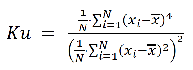
Now the kurtosis formula will be explained:

Where: 𝑥𝑖 is the i-th sample.
In the numerator of the fraction there is the calculation of the fourth statistical moment, while in the denominator there is the standard deviation elevated to the fourth power. Now the skewness formula will be explained:

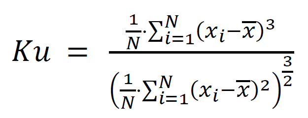
Where: 𝑥𝑖 is the i-th sample.
In the numerator of the fraction there is the calculation of the third statistical moment, while in the denominator there is the standard deviation elevated to the third power.

Again, as explained in the time domain algorithm, the decision of the statistical algorithm is based on the comparison between the statistical parameters and predefined thresholds that, if exceeded or not, a decision is then made.

Frequency Algorithm

The aim of this sub-algorithm is to detect signals in the frequency domain and eventually mitigate them by frequency blanking. This technique operates in a similar manner to Envelope Detection, but in the frequency domain. If a significant increase in power is observed at a particular frequency bin compared to its neighbouring bins, it may indicate the presence of interference. These power peaks are more easily detected when they have high power in a narrow bandwidth.

This analysis is done by comparing the received power from adjacent frequencies and applying a threshold to distinguish these values. So, if the algorithm detects a signal that is above that threshold, it decides that it is in fact an Interference.