ᴾᵒCat: Mission Analysis and Characterisations

• Mission analysis
• Mission analysis report
• Link and Data Budget Analysis
• Link budget
• Data budget
• Space Debris Mitigation
• Space Debris Mitigation report
• Characterisation and Calibration
• Solar cells
• Battery characterization test
• Battery degradation test
• Photodiodes Temperature Characterization
• Magnetorquer Polarisation verification
• Gyroscope Characterization and Calibration

Mission analysis

Mission analysis report

Mission analysis is a crucial aspect of space mission planning, involving a comprehensive review of satellite orbits and trajectory options to ensure the mission objectives are successfully met. This report presents the detailed mission analysis conducted for the project, which includes an evaluation of potential trajectory options, launch windows, and operational risks. The analysis spans the entire mission lifecycle, from initial concept to final operations, ensuring that all mission parameters are optimized for achieving the desired outcomes.

In this report, we will outline the findings of our mission analysis, including both baseline and alternative solutions, as well as the reasoning behind the selected trajectory. The comprehensive assessment provided here is designed to assist the project team in making informed decisions that align with the mission’s goals while ensuring safety, efficiency, and success in space operations.

Mission requirements and constraints

Objectives

The mission's objective is to collect data on Radio Frequency Interference (RFI) at L-Band and K-Band across the entire globe using PocketQubes, one dedicated to each frequency band, while also also disposing of another PQ capturing images of Earth with a VGA camera. Ideally, we aim to study a significant portion of the Earth's surface to gain a comprehensive understanding of global interference patterns. This requires certain orbital inclinations to be more suitable for observing higher latitudes. However, the mission has been designed with flexibility in mind, enabling the satellites to be launched under a variety of conditions.

Considerations

However, considering the type of satellites we will be using and the guidelines set by ESA’s FYS4!, there are still several factors to address. These include ESA’s Space Debris policy, explained in the Space Debris Mitigation report and the constraints outlined in the Link Budget.

Orbit compatibility

The following section details the results of our mission analysis, focusing on achieving maximum adaptability while adhering to the Space Debris policy and link budget constraints.

Altitude Range

For this part of the mission we need to consider the following factors:

ESA Zero Debris Approach

According to ESA Zero Debris Approach, the duration of orbital decay must be less than 5 years. As stated in the Space Debris Mitigation report, this requirement can only be met at specific altitudes and launch dates. The SDM report suggests that the optimal altitude should be between 450 km and 550 km.

Link Budget limitations

As outlined in the Link Budget provided for the Satellite Project File, the altitude impacts the free space losses encountered during the mission. Analyzing the three scenarios studied, communication is feasible in both the favorable and nominal scenarios (500km altitude). However, communication becomes more challenging in the adverse scenario. Taking into consideration these limitations we conclude that the optimal altitude range for our mission is from 450 km to 550 km.

Orbit Inclination

Two factors need to be taken into account selecting the orbit inclination:

Earth observation

The primary factor to consider is the mission’s purpose. As stated at the beginning of this report, our objective is to collect data on Radio Frequency Interference (RFI) at L-Band and K-Band and images (VGA) globally, which requires the satellites to regularly pass over most regions of the world. Based on fundamental orbital mechanics, this can only be accomplished at higher inclinations (80 to 100 degrees).

Minimum number of passes over GS

A minimum number of passes over the ground station (GS) must be taken into account. For example, as outlined in the Link Budget Analysis, with typical Earth observation inclinations (80 to 100 degrees), there is at least two to three communication pass per day.

In conclusion, the optimal orbit inclination for our mission should be between 80 and 100 degrees, ideally as close to a Polar orbit as possible to ensure global coverage. However, adaptability is a crucial aspect of our mission. Therefore, lower inclinations, such as the ISS inclination of 51.6 degrees, can also be considered. This inclination still covers a significant portion of the Earth, allows for five passes per day, and provides the opportunity to deploy the PocketQubes from the ISS.

Additional aspects

Eccentricity: Near zero, circular orbit.
SSO: Not required.
RAAN/LTAN: No preferences.

Link and Data Budget Analysis

Link budget

Introduction

A link budget assesses the various gains and losses that impact signal transmission from the satellite to the ground station, ensuring the communication link meets performance requirements.

By analyzing key factors such as transmission power, antenna gains, path losses, and atmospheric attenuation, we predict the signal-to-noise ratio (SNR) and system reliability. This revised document details the methodology, assumptions, and calculated outcomes, providing a comprehensive understanding of the system’s performance and limitations. These results are essential for validating the design and ensuring reliable data transmission for the IEEE Open PocketQube Kit mission. Please check the data budget for additional information regarding COMMS budgets.

Methodology

The methodology for calculating the link budget involves several key steps. First, we generated separate tables for each type of link: uplink and downlink. For each link, three different scenarios were considered: nominal, adverse, and favorable.

• Nominal scenario: Normal operation and conditions.
• Adverse scenario: Worst expected performance.
• Favorable scenario: Best possible performance.

It is important to note that all scenarios are calculated at a fixed orbit altitude of 500 km. The adverse and favorable scenarios have been updated to assess the variability of other parameters, such as antenna gain and losses. Additionally, we have revised the valid link margin for the nominal scenario to 3 dB for an orbit altitude of 500 km. Finally, calculations for the −3σ and RSS worst case have been performed using the adverse and favorable scenarios.

Parameter	Value	Description
Central Frequency [MHz]	868
Bandwidth [kHz]	125
Spreading Factor	11
Orbit Height [km]	500	Fixed altitude as per the Mission Analysis calculations.
Maximum Transmitted Power [dBm]	22	Maximum transmitted power as specified in the transceiver datasheet (SX1262).
Gain of the Monopole Antenna [dBi]	4	A quarter-wavelength monopole antenna has a gain of 5.15 dB. To account for a safety margin, we assume a gain of 4 dBi for the antenna.
Gain of the Patch Antenna [dBi]	12	Gain of the GS Yagi antenna as specified in the datasheet.
Polarization Losses [dB]	3	3 dB as we are using circular polarization.
Losses Due to Atmosphere [dB]	2	According to ITU-R recommendation 618, atmospheric losses are very small, primarily due to ionospheric scintillation. Also, ITU-R P.840-8 shows negligible attenuation due to clouds and rain at 868 MHz. Atmospheric losses are considered to be 2 dB.
Losses Safety Margin [dB]	3	As recommended in one of the RIDs, a link margin of 3 dB is applied.
Sensitivity for SF=11 [dBm]	-134.5	Given our bandwidth and spreading factor, our sensitivity is -134.5 dBm.
Sensitivity for SF=11 [dB]	-17.5	SNR sensitivity is -17.5 dB.

Please note that the gain of the quarter-wavelength monopole antenna shown in the table is 4 dBi. The theoretical gain of a quarter-wavelength monopole antenna is based on the gain of a half-wave dipole antenna, which is approximately:

Since a quarter-wavelength monopole antenna radiates only over half of the space due to the presence of a ground plane, its gain increases by 3 dB. Therefore, the gain of the monopole antenna is given by:

To incorporate a safety margin in our calculations, we assume a gain of 4 dBi for the quarter-wavelength monopole antenna.

Study cases

This section introduces each one of the scenarios that will be used for this link budget.

Favorable Scenario	Nominal Scenario	Adverse Scenario
500 km orbit height	500 km orbit height	500 km orbit height
0dB pointing losses	0.5dB pointing losses	1dB pointing losses
5.15dBi antenna gain	4dBi antenna gain	0dBi antenna gain (no deployment)
3dB link margin	3dB link margin	3dB link margin

Analysis of the results

This section presents the results from the Link budget analysis, detailing the findings for each study case across all three scenarios.

Power and SNR requirements

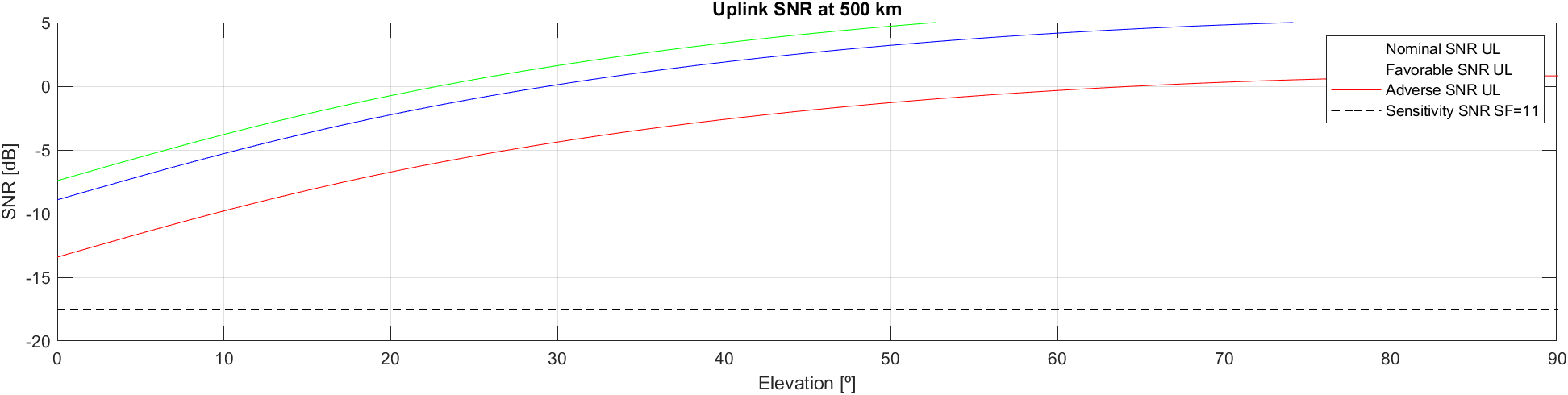
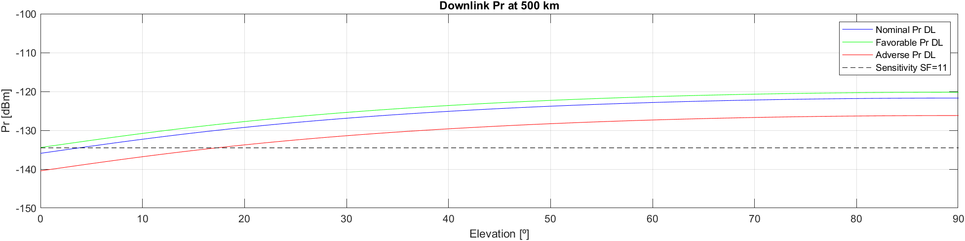
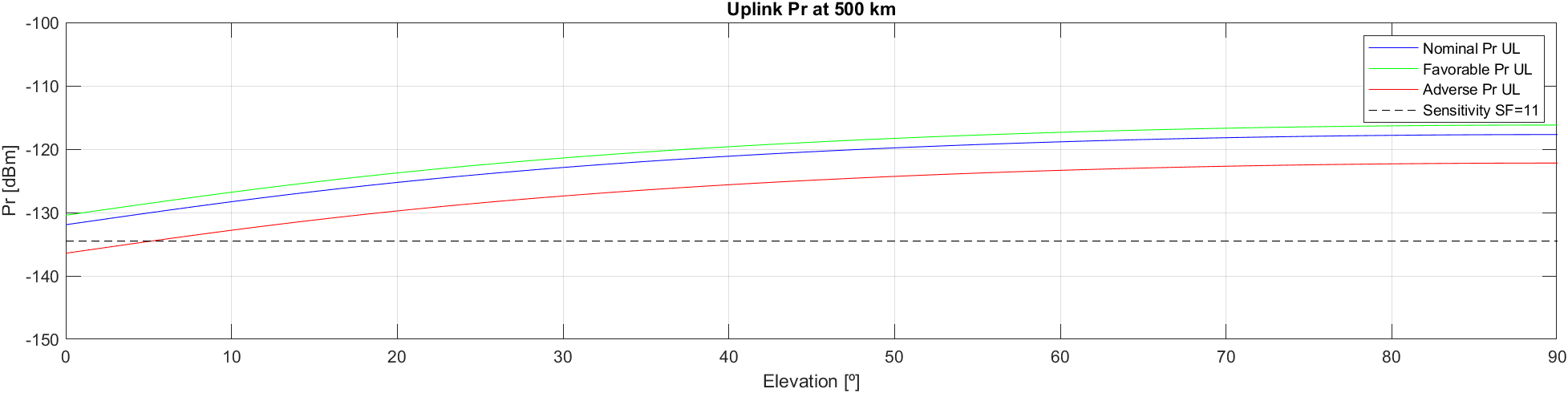
After running the code we created to compute the link budget, we have generated Figures shown below. These figures display the received powers for both Downlink and Uplink at each edge, as well as the corresponding SNR values. Note that the sensitivities outlined in the previous section are also represented as lines in the plots. The analysis of these results will determine the minimum elevation angle required for contact, identified by the intersections between the thresholds and the received power or SNR. A summary of the results is presented in this table:

Scenario		Favorable		Nominal		Adverse
		Prx	SNR	Prx	SNR	Prx	SNR
Downlink [min elevation angle]		0	0	4	0	17	1
Uplink [min elevation angle]		0	0	0	0	5	0

Conclusions

Once the link was computed, we looked for the references on the LoRa to demonstrate the disability of the link despite having a negative SNR [1]. Also, the approach to use LoRa on our mission was due to a recommendation from our professor, as the theoretical feasibility was demonstrated in [2]. To conclude, in addition to some experiments, [2] helped us to choose SF =11 and BW = 125 kHz.

1. Favorable Scenario:
   - Both uplink and downlink communications are highly reliable.
   - Minimum elevation of 0°, ensuring robust communication links.
2. Nominal Scenario:
   - Taking into account an antenna gain of 4dBi and a link margin of 3dB as recommended by ESA's expert.
   - Communications remain reliable, though with slightly higher minimum elevation angles (4° for downlink and 0°
   for uplink).
   - Communications are feasible but require more optimal conditions compared to the favorable scenario, especially
   for the downlink.
3. Adverse Scenario:
   - Taking into account no antenna deployment as well as worst system performance.
   - Uplink communication is possible but requires minimum elevation of 5°.
   - Downlink communication is possible but requires minimum elevation of 17°.

In our analysis, we calculated the −3σ margin, which provides a conservative estimate of the link performance under adverse conditions. The calculated −3σ margin was found to be 4.9505, indicating the minimum acceptable performance level for reliable communication.

Additionally, the worst-case RSS analysis yielded a total RSS of 3.4689. This worst-case scenario confirms the robustness of our system, with a link margin superior to 0 dB, as it demonstrates the ability to maintain communication links even under challenging conditions.

Both parameters were calculated as detailed in ECSS-E-ST-50-05C, section 8.

The link budget analysis demonstrates the feasibility of our communication system for the PoCat Lektron mission PocketQubes, developed under ESA’s FYS4! program. The analysis considers different scenarios for uplink and downlink communications, including favorable, nominal, and adverse conditions.

Moreover, when taking adverse conditions, we find that communication is possible even in challenging scenarios. This confirms the link’s feasibility.

References

[1] RF Wireless World. LoRa Sensitivity Calculator. https://www.rfwireless-world.com/calculators/ LoRa-Sensitivity-Calculator.html, 2024.

[2] L. Fernandez, J. A. Ruiz-De-Azua, A. Calveras, and A. Camps. Assessing lora for satellite-to-earth communications considering the impact of ionospheric scintillation. IEEE Access, 8:165570–165582, 2020.

Data budget

Introduction

This document outlines the methodology, assumptions, and calculated results, providing a clear understanding of the system’s data management and limitations. These results are crucial for validating the design and ensuring reliable data transmission for the IEEE Open PocketQube Kit. Please check the link budget for additional information regarding COMMS budgets.

Methodology

As detailed in the link budget, the simulated nominal scenario for obtaining values and performing computations involves an orbital height of 500 km.

To determine the data budget, we need to calculate the maximum amount of data that can be downloaded in a single pass. This requires computing the capacity for a Spreading Factor (SF) of 11 and a Code Rate (CR) of 4/5. Using the formulation provided in [1], we obtain a rate of 537.11 bps.

After obtaining the data rate, we propagated the orbits using Orbitron [2] to study the initial scenario. This software has an inclination error of 0.1º. The propagation results provided the satellite passes over the Ground Station (GS) at Montsec [3], factoring in the minimum elevation angle. Using the simulated pass durations and the calculated data rate, we calculated the data that can be transmitted during each pass over our ground station. 

We then compared the average data that can be transmitted in uplink and downlink with the required data for sending commands from the satellite and the GS. We verified that the available data was sufficient to transmit and receive telecommands and payload results, and ensured that data could be re-sent if needed, as there are no protocols guaranteeing packet reception.

The table below estimates the total data volume needed for transmission during each satellite pass, covering both telemetry/configuration data and payload data for a single measurement.

Downlink
Telemetry data	48 Bytes
Configuration data	32 Bytes
Payload 1 (L band) data	2831 Bytes
Payload 2 (K band) data	708 Bytes

This data will be stored inside the satellite with up to 1MByte of storage. For the uplink, we have a variety of telecommands available.

A detailed list of all telecommands, along with the corresponding telemetry, can be found here.

Since the number of bytes required for the uplink will largely depend on the amount of available platform data and the satellite’s latest status, estimating the exact byte count for the uplink is impractical.

However, as indicated in the summary table, the PocketQubes will have a large margin, ensuring that even in a worst-case scenario—where a significant number of commands need to be uploaded during a pass—there will be sufficient time to do so.

Results

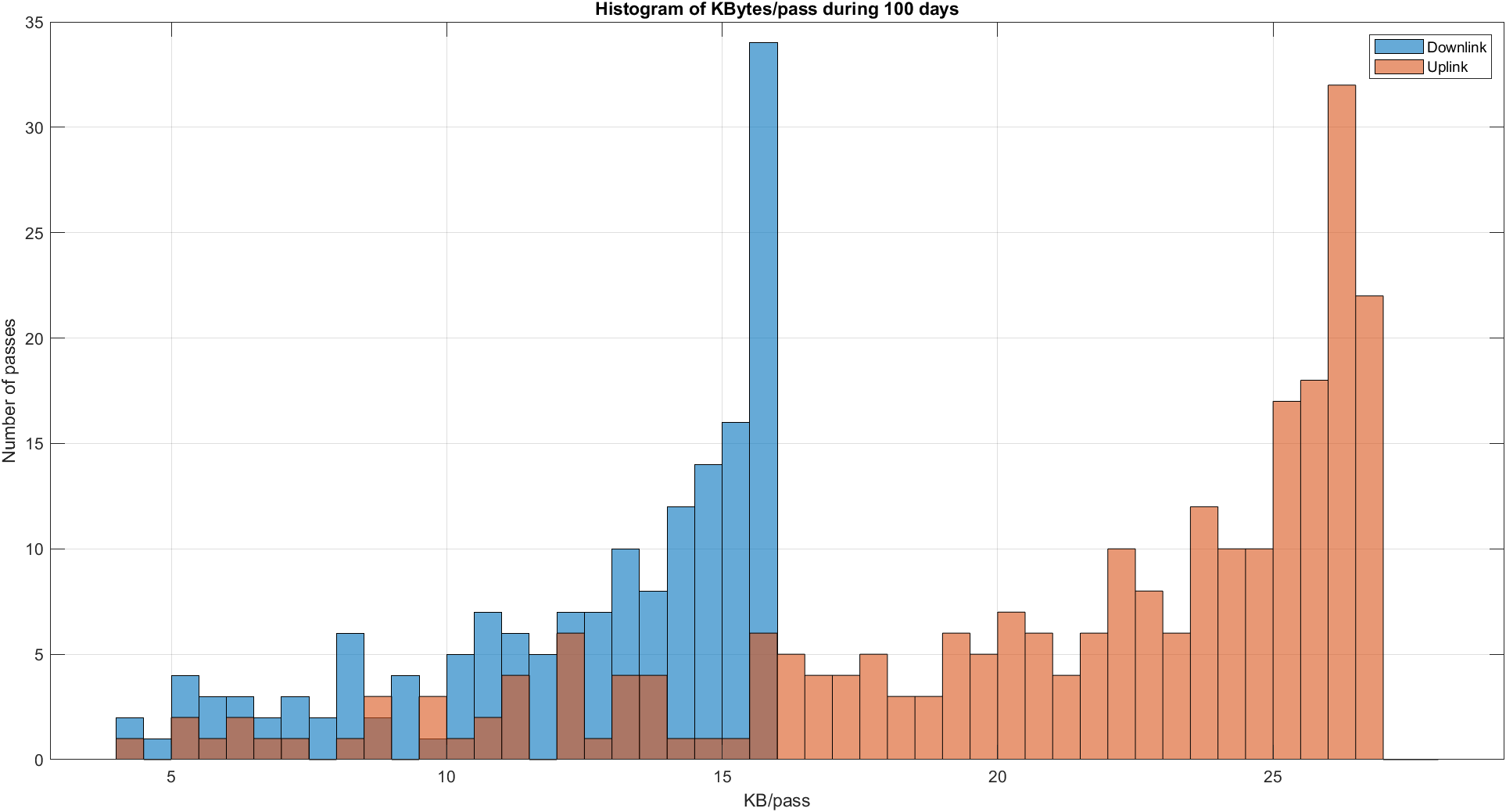
This section presents the results from the Data budget analysis. First, we have computed the number of passes available with its corresponding duration. Figure below shows the number of passes according to its duration for both uplink and downlink in 100 days:

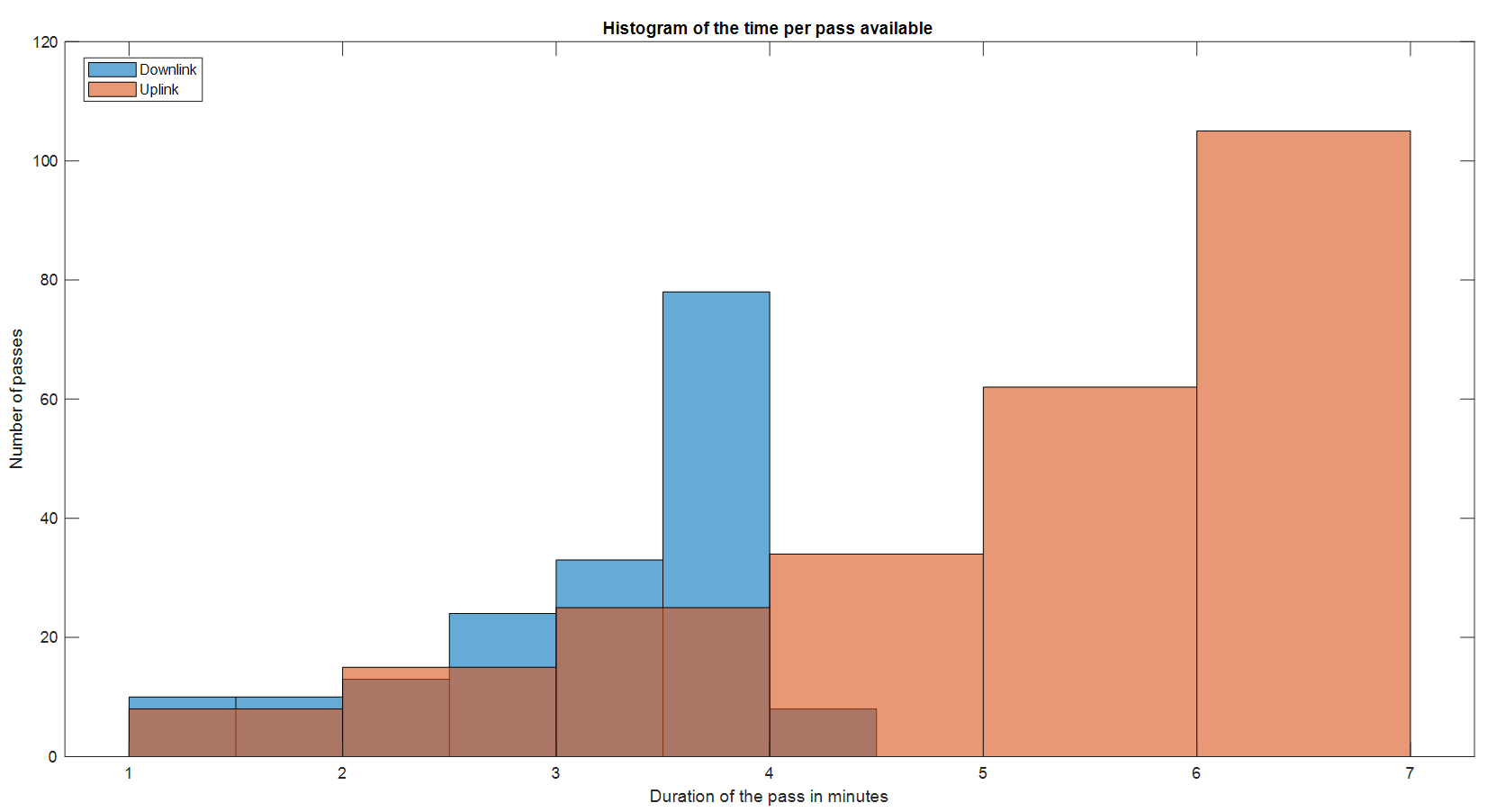
After obtaining the results from Figure G.5, we can compute the data that can be sent during each pass based on the findings presented in [1]. On average, we have 2.49 uplink passes per day over a period of 100 days. For the downlink, we achieve about 1.63 passes per day. Table below presents the results, showing the average duration of the passes for both uplink and downlink.

Average pass time [min]
Uplink	5.26
Downlink	3.18

The data was obtained by multiplying the rate by the time per contact, resulting in the outcomes shown in the Figure below. This figure displays the amount of data available for download per pass, revealing the number of contacts related to the downloaded data. To summarize the findings from the Figure below, tables are provided, offering an overview of the average data downloaded per pass using the results from the Table above. The presented results indicate the data downloaded per pass and per day.

Average transmitted Bytes per pass [kBytes]
Uplink	20.69
Downlink	12.52

Average transmitted Bytes per day [kBytes]
Uplink	52.05
Downlink	22.26

From the results in the Tables above, we can now gauge the link’s capabilities for downloading data. Lastly, Figure below illustrates the kBytes per pass in relation to the maximum elevation angle the satellite reaches during that pass, which directly correlates with the maximum data we can download.

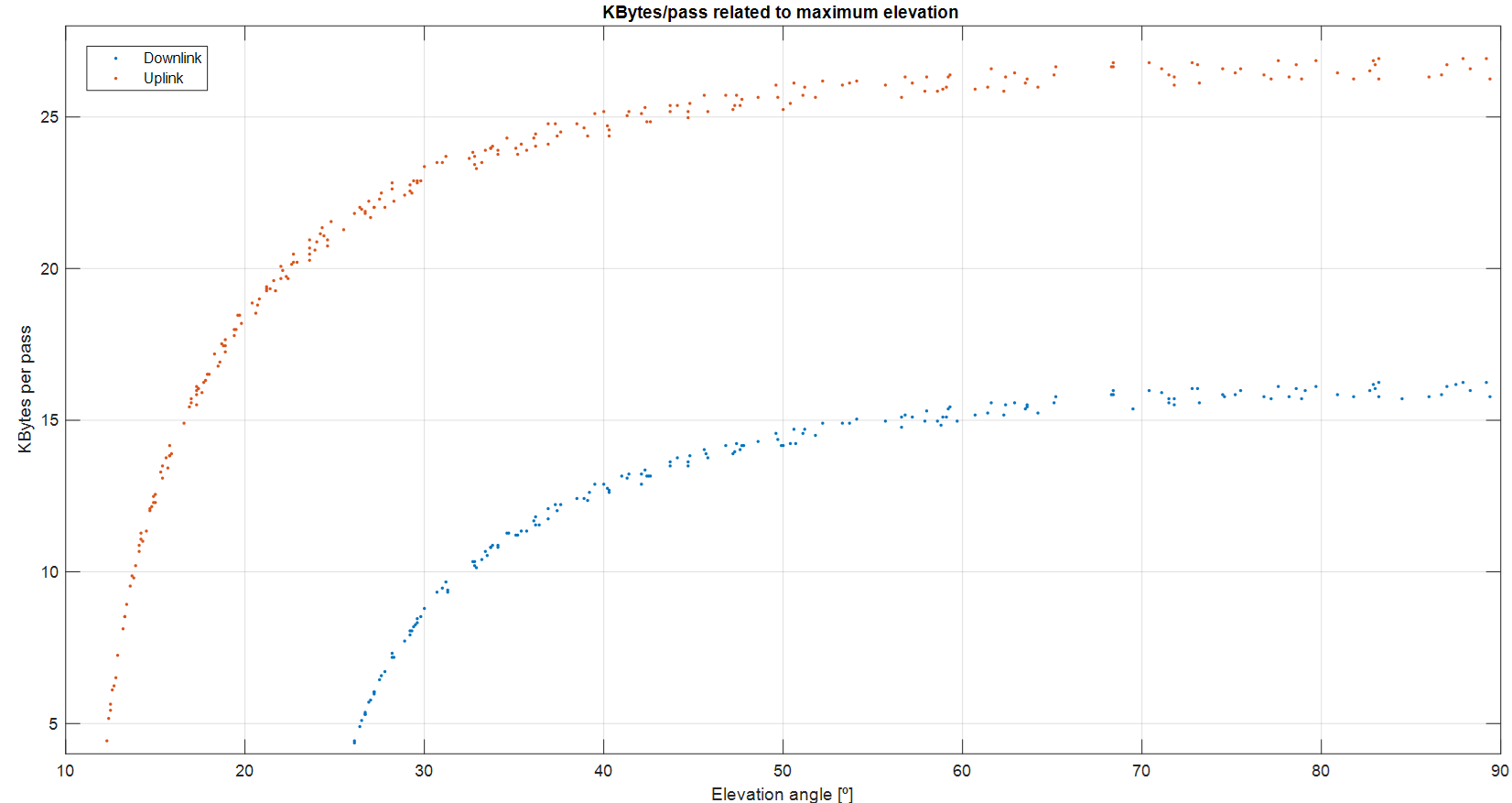
Analyzing the results, we find that the uplink transmission capacity is 20.69 kBytes. For the downlink case, the transmission capacity is 12.52 kBytes, while the L-band payload (which is the payload generating more data) requires 2831 Bytes (2.76 kBytes) to be downloaded from the satellite to the ground station. Therefore, we can conclude that the data budget capabilities are sufficient and that additional stored data could also be transmitted from the satellite to the ground station.

Conclusions

Table below demonstrates our capability to transmit at least one image per contact. Additionally, telemetry data can be sent along with the image once per pass. Furthermore, we have the ability to repeat messages if necessary to ensure successful transmission.

	Maximum Data Volume capability per pass [Bytes]	Estimated Data Volume to be transmitted [Bytes]	Additional available Bytes	Feasibility
Uplink	21191	x	20567	TRUE
Downlink PL1	12824	2831	9993	TRUE
Downlink PL2	12824	708	12116	TRUE

Additionally, following the recommendation of ESA’s expert, we present a demonstration of the data budget’s feasibility, factoring in the time required to transmit all the data. Specifically, the airtime for each packet will be approximately 1478 ms [4].

By adding a few seconds for computation time and a margin of error and considering an average pass, we arrive at:

	Data to be transmitted [Bytes]	Time required to transmit data [s]	Time left [s]	Feasibility
Uplink	500*	18.5 (+2) = 20.5	295.1	TRUE
Downlink PL1	2873	106.2 (+2) = 108.2	82.6	TRUE
Downlink PL2	708	26.2 (+2) = 28.2	162.6	TRUE

It can be observed that both PocketQubes will have sufficient time to communicate and transmit all the necessary data to the ground station, confirming the feasibility of this data budget.

* It is important to note that for the uplink, we have selected a data size of 500 bytes for transmission. As mentioned earlier, the exact amount of data required for the uplink will depend on various factors.

References

[1] RF Wireless World. LoRa Sensitivity Calculator. https://www.rfwireless-world.com/calculators/ LoRa-Sensitivity-Calculator.html, 2024.

[2] Stoff Industries. Orbitron - Satellite Tracking System - Official Website. https://www.stoff.pl/ , 2024. 

[3] Parc Astronòmic Montsec. Parc Astronòmic Montsec. https://parcastronomic.cat/es/ , 2024

[4] The Things Network. The things network airtime calculator. Online Tool, 2024.

Space Debris Mitigation

Space Debris Mitigation report

Introduction

This report focuses on space debris mitigation for PocketQube satellites as part of ESA’s FYS4! program. Space debris includes defunct satellites, spent rocket stages, and other fragments orbiting the Earth. As the number of satellites and space missions increases, the risk of collisions and further debris generation also rises. Effective mitigation strategies are crucial for ensuring the long-term sustainability of space activities. PocketQube satellites have gained popularity due to their compact size and low cost. However, their small size makes implementing effective debris mitigation measures challenging. This report addresses these challenges and proposes strategies to minimize debris creation during the operational phase of PocketQube satellites. Given that PocketQubes lack propulsion systems, the report suggests launching them at low altitudes to ensure an orbital decay of less than five years, aligning with ESA’s Zero Debris policy. By analyzing current space debris mitigation practices and considering the specific requirements of PocketQube satellites, this report provides recommendations for launching and operating these satellites to minimize their contribution to space debris. The findings and recommendations in this report will promote sustainable space activities and reduce space debris risks. Implementing these mitigation measures aims to ensure the long-term viability of PocketQube satellites and contribute to a cleaner, safer space environment.

Mission profile

As outlined in the Mission Analysis Report , the ideal altitude range is between 450 km and 500 km, with an orbital inclination close to Polar, which is optimal for Earth observation. While lower inclinations are also feasible, aim for an eccentricity near zero. For further details, please consult the Mission Analysis Report.

Mission requirements

As noted in the Mission Analysis Report, the mission does not have any strict limitations. However, altitudes above 500 km and low orbital inclinations may pose challenges for communication with our ground station located at the Montsec Observatory in Lleida.

Satellite space system description

Overview

Each of the satellites will be equipped with a range of systems, with the only difference being the payloads they use. The structural design is outlined in the Satellite Project file’s Structure section. The other systems include the Power System, On-Board Computer, Telemetry, Tracking, and Communication System, Attitude Determination and Control System, and Payload Systems (VGA, L-band, K-band), along with additional subsystems related to these major components.

Power system

• Energy Harvest Block:
  – Includes 3 Maximum Power Point Trackers (MPPTs) to optimize energy generation from the solar cells.
  – Equipped with 5 high-efficiency GaAs triple junction solar cells with an efficiency of over 30%.
  – Two solar cells are placed in parallel on the X and Z axes, and one on the Y-axis.
• Battery Charger Block:
  – Manages energy and charges a 3.7V, 1400mAh LiPo battery.
  – The power management IC monitors the battery and communicates with the On-Board Computer (OBC)
  to adjust operations based on voltage, current, temperature, and capacity.
  – Equipped with an NTC temperature sensor and a heater for battery temperature regulation.
  – A voltage regulator reduces the battery voltage to 3.3V for the subsystems.
• Killswitches:
  – Killswitches keep the satellite powered off on Earth and activate once in space, connecting the battery to
  the satellite.

Attitude and Orbit Control System (AOCS)

The AOCS will determine the orientation of the satellite in two different scenarios, the first one with direct sun exposition, and the second one without direct sun exposition. In order to obtain the information from the environment it will use a gyroscope and a magnetometer. In addition, it will also use photodiodes and temperature sensors installed on the spacecraft’s lateral boards. Regarding spacecraft control, as detailed in the ADCS section, the only control mechanism available will be orientation adjustment via magnetorquers. These magnetorquers are embeeded in each lateral board and in the bottom board. In the case of the +Y magnetorquer, it is located in an inner PCB inside the Pocketqube structure. The main functionalities of the AOCS are nadir pointing to point the payload at the nadir angle, and the detumbling, to reduce the rotation of the satellite. Regarding the requirements for between the AOCS and the communications antenna, as it is a monopole it does not require any pinting accuracy. For the spacecraft navigation the on board computer will propagate the orbit and estimate the current position of the satellite around the Earth.

Implementation and verification

Mission related objects (MROs)

No objects will be realised from the PocketQubes at any point of the mission.

Small particle release

Similar to the previous sections, the satellites do not have a propulsion system; therefore, no particles larger than 1 mm are expected to be released.

Additionally, the dyneema used for deploying satellite antennas, such as the communication and payload antennas, is designed to remain attached to the satellite after the antenna deployment is completed.

On-orbit break-up risk caused by the system

Due to the compact size of the PocketQubes, especially within the deployer, no fragile elements have been used, minimizing the risk of breakage. Additionally, the satellite’s structure is assembled with screws, which are further secured by helicoils.

Regarding the lateral boards, epoxy is applied to keep the solar panels securely attached to the satellite. The photodiodes on the lateral boards must also pass a vibration test before launch, making the likelihood of breakage extremely rare.

On-orbit collision risk

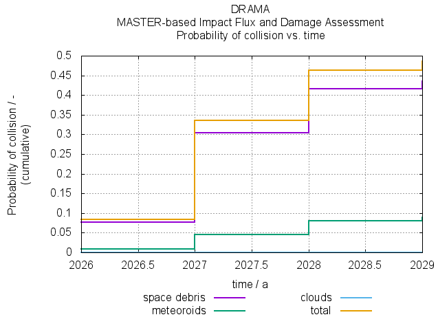
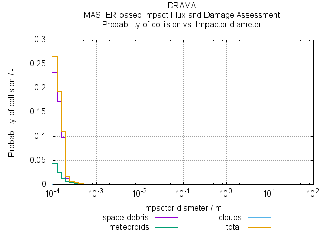
To analyze the on-orbit collision risk of our platform, the MIDAS tool from DRAMA was utilized. The simulations account for a launch scheduled in Q3 2026 with a mission duration of 3 years, adjust your values to the expected launch date.

The following spacecraft parameters were applied:

Parameter	Value
Semi-major axis [km]	6871
Cross-sectional area [m^2]	0.005
Drag coefficient	2.2
Mass [kg]	0.234
Solar radiation pressure reflectivity coefficient	1.2

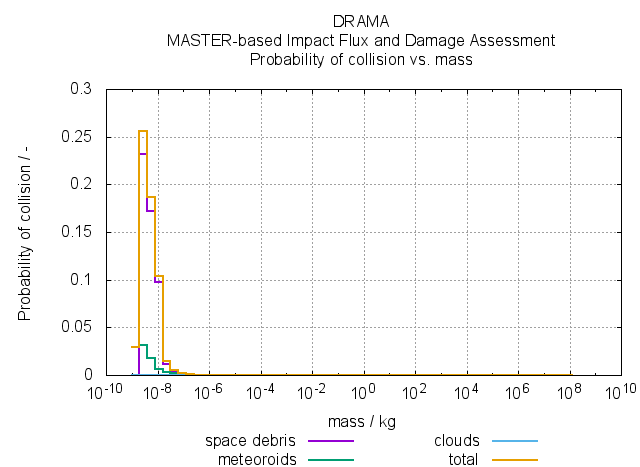
To provide a comprehensive overview of the collision risk, three key figures are presented. The first graph illustrates the probability of collision as a function of time throughout the mission duration. Second graph shows how the spacecraft’s mass impacts the probability of collision, while third graph demonstrates the effect of the spacecraft’s diameter on the collision likelihood.

These figures collectively highlight the main factors influencing the on-orbit collision risk:

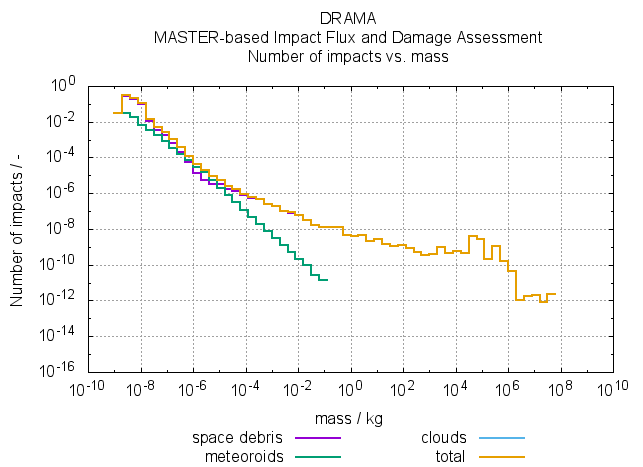
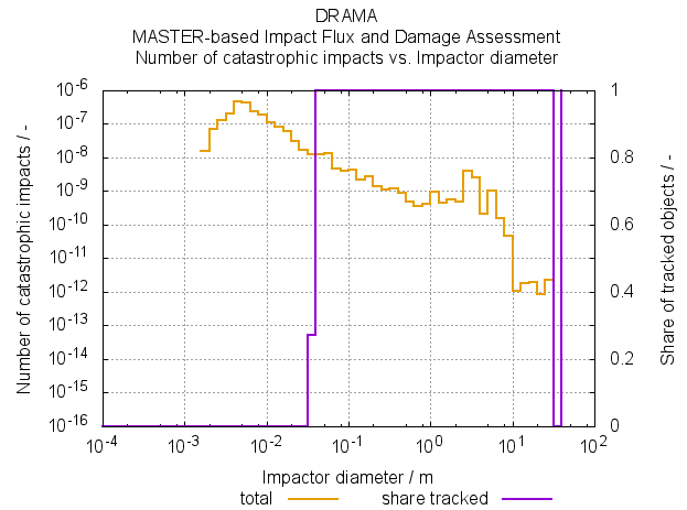
On-orbit break-up and vulnerability risk caused by impacts

Similar to the approach taken in the previous section, the MIDAS tool from DRAMA was used to analyze the on-orbit break-up and vulnerability risks due to impacts on our platform. The simulations consider a launch planned for Q3 2026, with a mission duration of 3 years.

Parameter	Value
Semi-major axis [km]	6871
Cross-sectional area [m^2]	0.005
Drag coefficient	2.2
Mass [kg]	0.234
Solar radiation pressure reflectivity coefficient	1.2

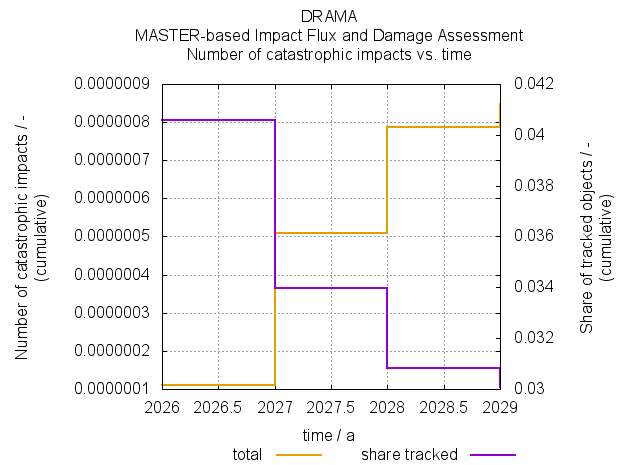
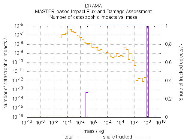
To further analyze the on-orbit collision risk, six additional graphs are introduced. The fourth, fifth, and sixth graphs show the number of impacts over time, as well as the influence of mass and diameter on the number of impacts, respectively. The seventh, eighth, and ninth graphs illustrate the number of critical impacts, again as a function of time, mass, and diameter. These graphs provide a deeper understanding of both the total number of impacts and the severity of critical impacts across various parameters.

Disposal

Due to the design of our satellite, it lacks a propulsion system. Consequently, both of our PocketQubes will reenter the atmosphere uncontrollably once orbital decay causes them to descend enough. The following orbital propagation analysis estimates the expected mission lifetimes based on three scenarios with varying initial altitudes. These simulations were performed using ESA's "OSCAR" tool, part of the DRAMA software package. A detailed list of the parameters used is provided below:

Parameter	450km scenario	500km scenario	550km scenario
Semi-major axis [km]	6821	6871	6921
Eccentricity	1.00E-04	1.00E-04	1.00E-04
Orbit inclination [º]	98	98	98
Cross-sectional area [m^2]	0.005	0.005	0.005
Drag coefficient	2.2	2.2	2.2
Mass [kg]	0.234	0.234	0.234
Solar radiation pressure reflectivity coefficient	1.2	1.2	1.2

The semi-major axis values correspond to the scenarios mentioned earlier, which are also used in the Link Budget and assume possible initial orbit altitudes of 450 km, 500 km, and 550 km. A near-zero value has been selected for the eccentricity. For the cross-sectional area and coefficients, worst-case scenarios have been considered, as recommended by ESA experts. 

Lastly, it is important to note that these simulations are based on a projected start date in Q3 2026, which is our current mission launch target. The tenth, eleventh, and twelfth graphs show the satellites' altitude over time, along with the estimated mission duration. This means the launch date needs to be adjusted depending on the specific expected launch date.

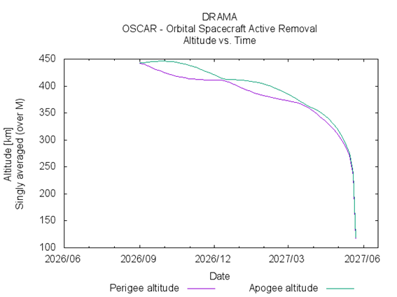
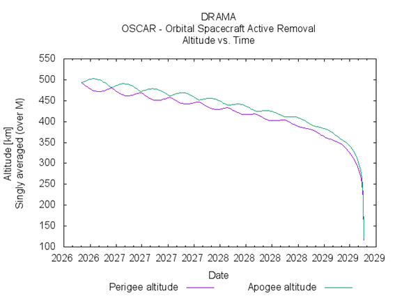
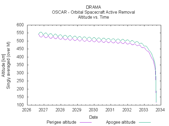
As seen in the three scenarios, initial altitudes below 550 km comply with ESA’s Zero Debris approach, while altitudes above 550 km do not meet the compliance criteria. In any case, launching at this altitude range would ensure that the satellites eventually reenter the atmosphere.

This considers the worst-case scenario where the antennas fail to deploy, resulting in a smaller cross-sectional area and therefore less drag than intended. Consequently, a deployment issue or satellite malfunction would not significantly impact the reentry time of the satellite.

Reentry

As outlined in earlier sections of the Space Debris Mitigation report, the constraints of the PocketQube mean that controlled reentry is not feasible. The mission does not plan for satellite recovery or reentry, so no heat shields or specialized designs have been employed to ensure the satellites’ survival during reentry.

Hazardous materials

The PocketQubes do not dispose of any fuel, as they do not have a propulsion system. However, they are equipped with a LiPo battery, which can be hazardous if exposed to extreme conditions. LiPo batteries can become explosive if damaged or overcharged, release toxic substances if breached, and pose a fire risk due to their flammable electrolyte.

Characterisation and Calibration

Solar cells

Datasheet and 3D model of our Ligtricity s3040_CIC solar cell https://satsearch.co/products/exa-solar-cells-30-40

This page states that it belongs to another company ‘Ecuadorian Space Agency (EXA)’ but the datasheet and 3D model correspond to the solar cell used in this Kit.

Battery characterization test

Test Description and Objectives

The objective of this test is to perform and analyse a charge cycle of the battery using the battery test equipment.

Requirements Verification

Requirement	Description
1	Battery can be completely charged
2	Battery can be completely discharged
3	Battery voltage shall be recorded during all the test duration
4	Battery current shall be recorded during all the test duration
5	Battery temperature shall be recorded during all the test duration
6	Total power charged to the battery shall be recorded

Test Set-Up

The test setup can be seen below

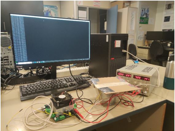
• Subsystem and its components
• Battery tests equipment.
• 2 power supply cables with bananas in both sides.
• 2 power supply cables with bananas in one side and exposed copper in the other one.
• Dual power supply or 2 independent ones.
• Flat small screwdriver.
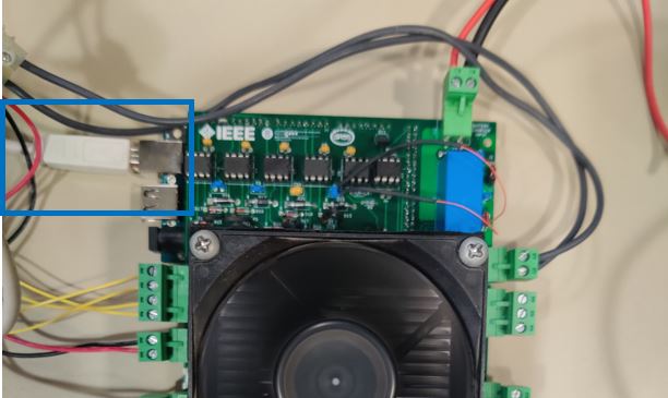
• USB A to USB B cable.
• Computer with the Arduino IDE and Putty Installed for data logging.
• Battery to be tested.
• 2,5 A Fuse and fuse holder.
• Some wire.
• Connectors to connect cable between them.
• Metal container for the battery.

Pass/Fail Criteria

This test is designed to characterize a charge cycle for the PocketQube battery. There is no pass or fail criteria as the result will be the charge curves of the battery. However, after having these curves, depending on the application, further study can be needed, in order to determine whether the battery is suitable for the desired task.

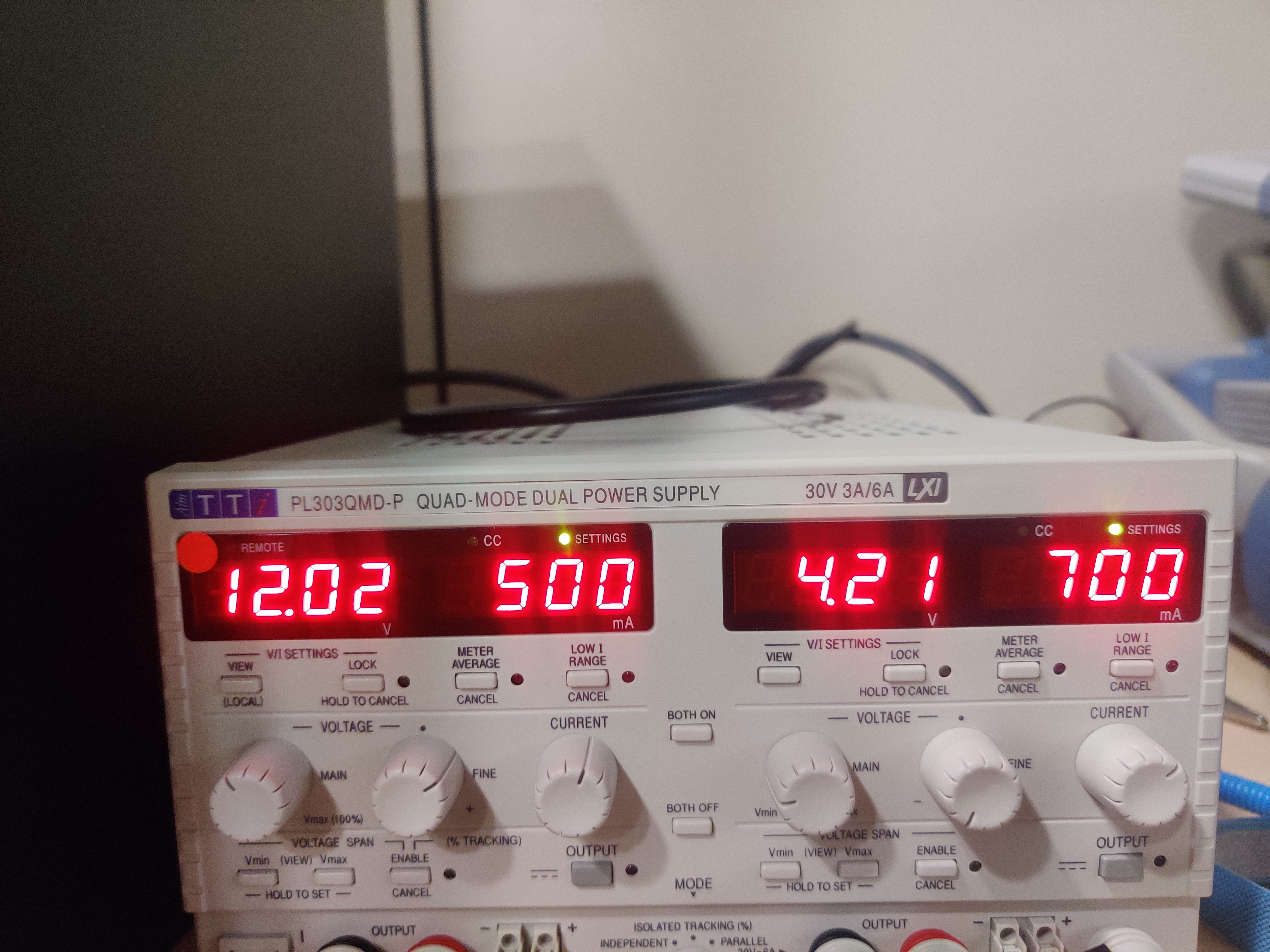
Test Plan

1. Regulate the power supply with one channel set to 12 V and 500 mA and the other channel set to 4,2 V and C/2 mA (current limit should be equal to half the battery capacity) 700 mA for this battery test.

2. Connect using 2 banana cables the 12V output from the power supply to the banana connectors from the battery test apparatus respecting the polarity. DO NOT ENABLE THE POWER SUPLY OUTPUT YET.

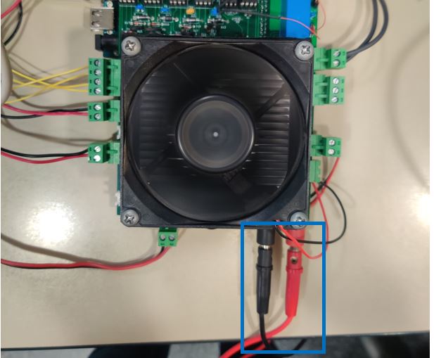
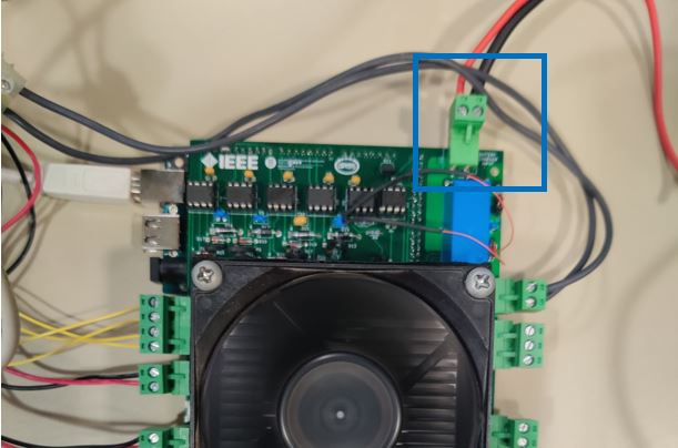
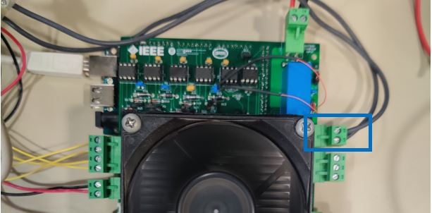
3. Connect the output from the 4,2V power supply to the top terminal block labelled as BATTERY CHARGE INPUT respecting the polarity. DO NOT ENABLE THE POWER SUPLY OUTPUT YET.

4. Attach the NTC to the battery under test using tape. Wrap it as tight as possible to ensure good contact between the NTC and the battery. The NTC that needs to be attached to the battery is the TOP one from NTC Battery 4 pin block terminal marked with a yellow dot on the block terminal.

5. Enable the 12V power supply output.

6. Connect the USB cable to the Arduino and PC and upload the charge .ino test code to the board. Select the adequate COM port on the Arduino IDE and remember it for the following steps.

7. Disconnect the USB cable from the PC.

8. Disable the 12V output.

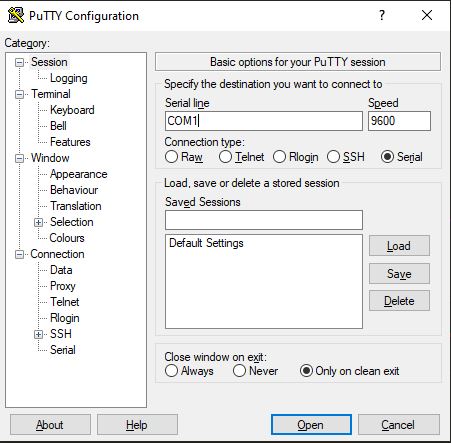
9. Open PUTTY and select connection type: Serial and write down the Arduino COM port previously indentified.

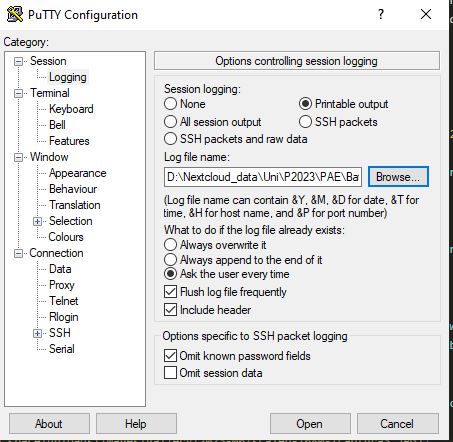
10. In PUTTY go to the Logging tab and select Printable Output and select the folder where you want to save the test data.

11. Connect the battery cables to the terminal block labelled as BATERY respecting polarity and installing a Fuse of 2,5A between the battery test apparatus and the battery.

12. Put the battery inside the metal container as a precaution measure in case of explosion.

13. Enable both power supply channels.

14. Connect the USB cable to the PC and click on Open on the PUTTY software.

15. If all steps were performed correctly, the text START ARDUINO will be visible, and, after pressing any key of the keyboard, the test will start. Every 5 seconds a new line will be written indicating the voltage, current, accumulated power and temperature separated by a semicolon (“;”).

16. Each cycle end will be indicated on screen and at the beginning of each charge cycle the test iteration will be written. At the end of the entire test, a “TEST END” prompt will appear. Note that for a test of 10 iterations will take approximately 3 days to complete.

17. Disconnect USB cable.

18. Turn off power supplies.

19. After that the data will be available in the folder you selected before, and you can use any software capable to graph and analyse the result data from the CSV file.

Test Results

This test was carried out at NanosatLab between 02/06/2023 and 05/06/2023 by Adrià Molló Carulla. The RAW data in CSV and also the processed data in an Excel file is attached to this document. This has been performed at ambient temperature (cca 25C). While already a good breakthrough, if time allows, a hot (40C) and cold (4C) case should also be performed for at least 5 cycles.

Frome the test the following results have been obtained:

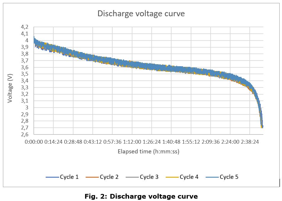
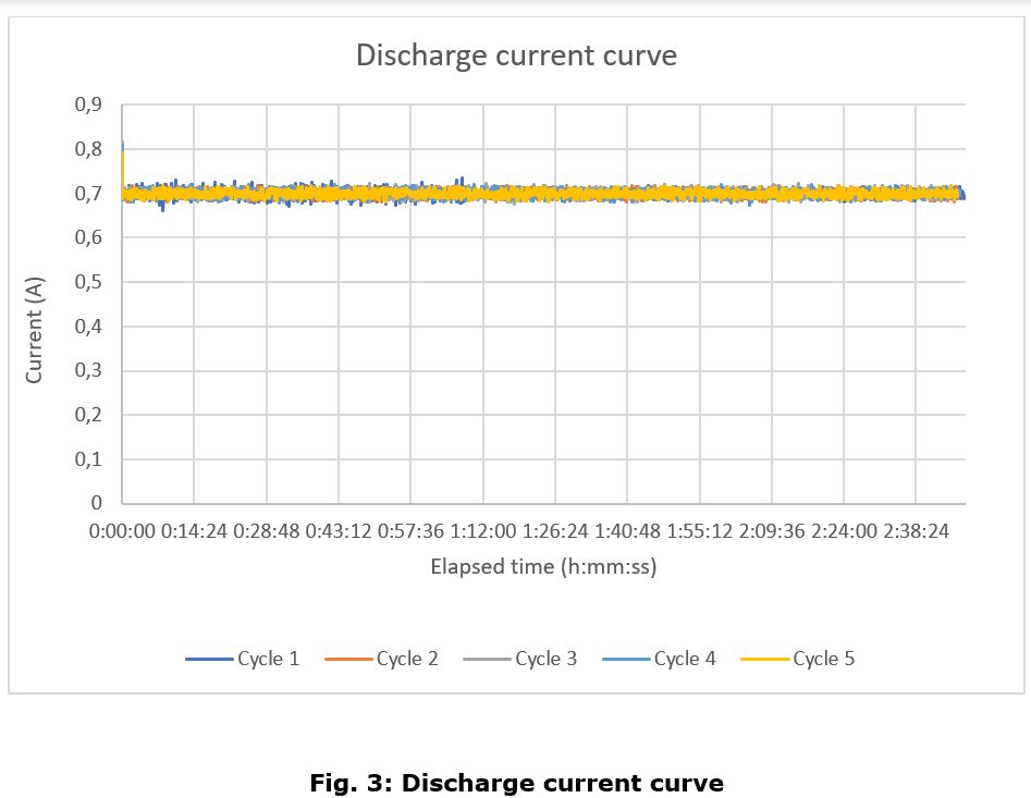
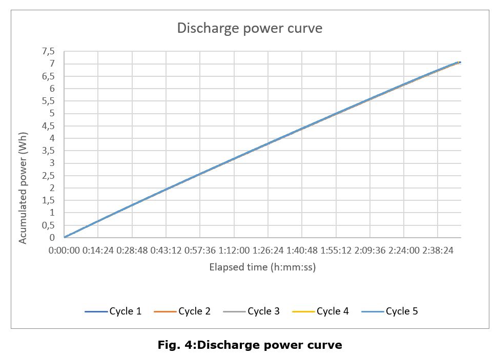
Discharge Cycle

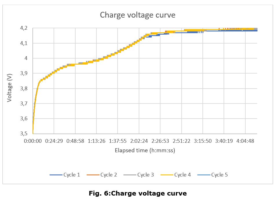
Charge Cycle

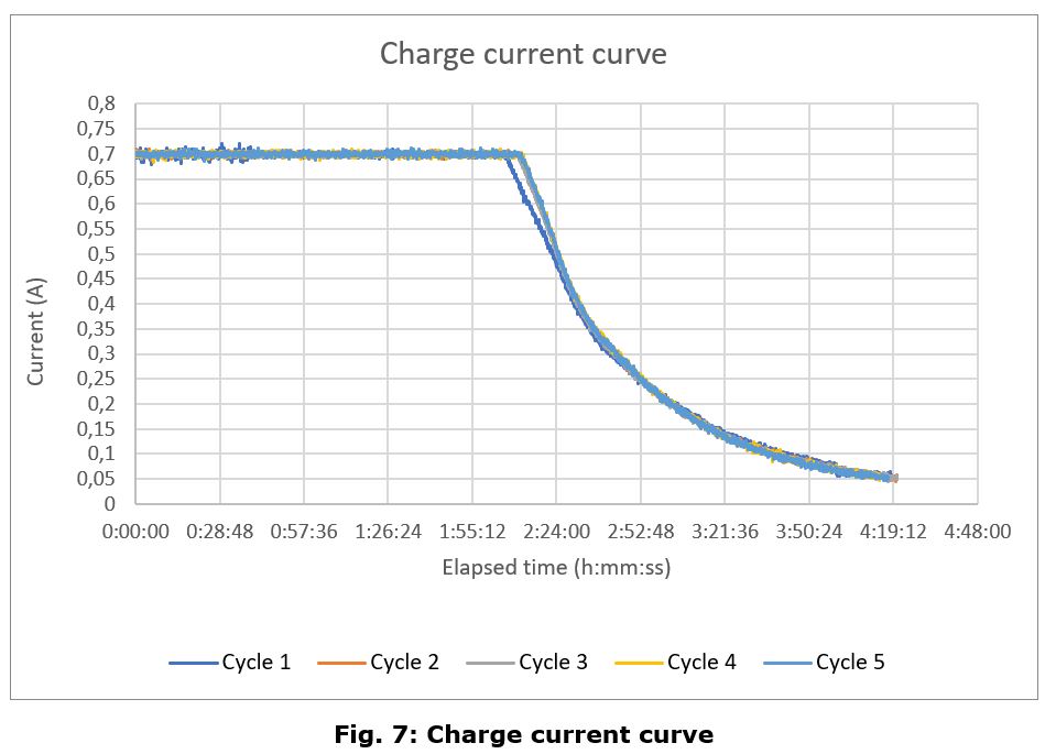
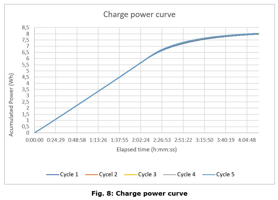
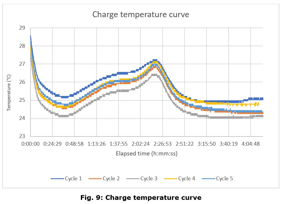
In Table 1 there is an overview of the main parameters of the battery for each iteration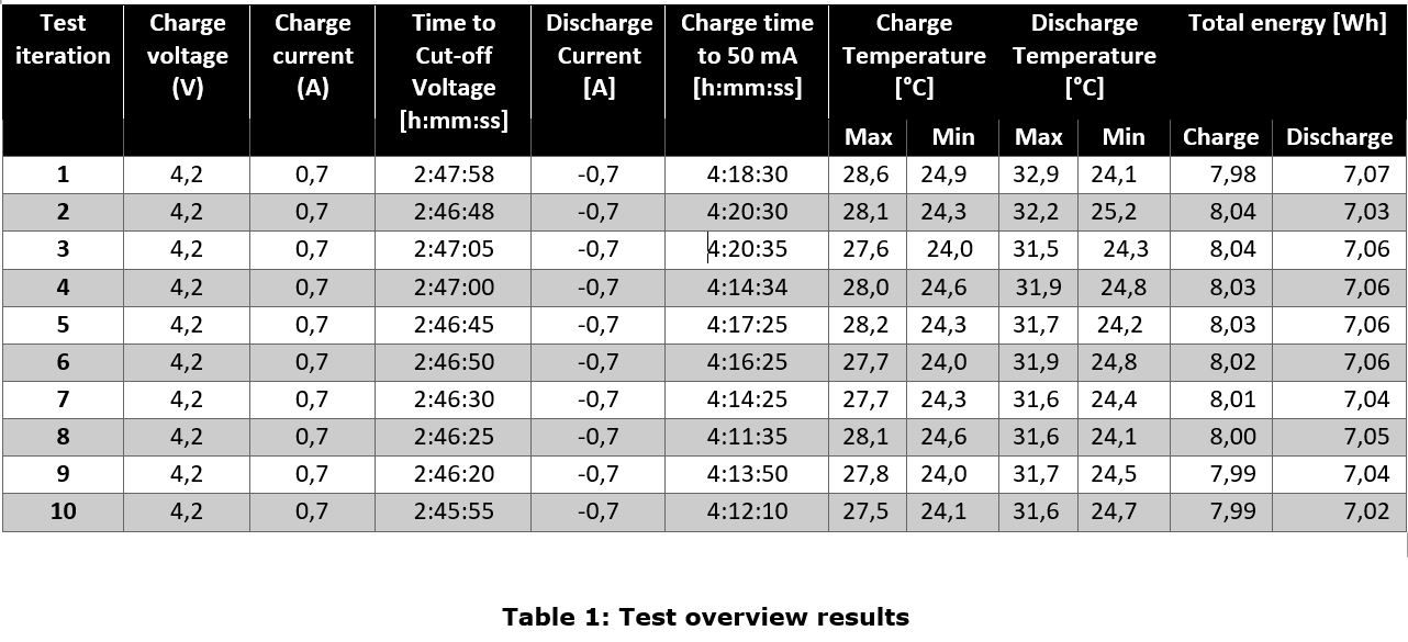

Anomalies

It has been found that the battery capacity appears to be considerably higher than the declared by the manufacturer (5,16 Wh) compared to the tested one (7,07 Wh).

Conclusions

The main conclusions of this test campaign are that the battery charge and discharge curves look follow the same pattern as a generic lithium polymer battery, with no appreciable differences, except for the aforementioned anomaly.

The full test code is available at: 

Link broken, to be inserted.

Battery degradation test

Test Description and Objectives

The objective of this test is to perform and analyse the degradation of the battery in LEO orbit thermal conditions.

Due to time constraints, in order to see the proper degradation of the battery, a full charge and discharge of the battery will be carried out. That is, charging to 4.2V and discharging till 2.7V at a rate of C/2 mA. As to the temperature conditions, the same logic has been followed. The charging cycle will be done at the highest possible working temperature (40ºC) and a moderate 10ºC for the discharge cycle (instead of the lowest 2ºC). This configuration has been adopted because the battery will normally be charged by the solar panels when the PocketCube is facing the sun and discharged during the eclipse phase.

Requirements Verification

Requirement ID	Description
1	Battery can be charged
2	Battery can be discharged
3	Battery voltage shall be recorded during all the test duration
4	Battery current shall be recorded during all the test duration
5	Battery temperature shall be recorded during all the test duration
6	Total power charged to the battery shall be recorded
7	LEO thermal conditions must be simulated

Test Set-Up

• Subsystem and its components.
• Battery tests apparatus.
• 2 power supply cables with bananas in both sides.
• 2 power supply cables with bananas in one side and exposed copper in the other one.
• Dual power supply or 2 independent ones. One must be able to supply 12V and 6A the other one must be able to supply 4,2V and 1A.
• Flat small screwdriver.
• USB A to USB B cable.
• Computer with the Arduino IDE and Putty Installed to log data.
• Battery to perform the test one.
• 2,5 A Fuse and fuse holder.
• Some wire.
• Connectors to connect cable between them.
• Empty metal case for the battery.

Pass/Fail Criteria

This test is designed to characterize a degradation of the PocketQube battery over a great number of cycles and temperature ranges. There is no pass or fail criteria as the result will be the information pertaining to the charge and discharge curves of the battery.

Test Plan

1. Regulate the power supply with one channel set to 12V and 6 A and the other channel set to 4,2V and adjust the current limit so it matches the max desired charge current.

2. Connect with 2 banana cables the 12V output from the power supply to the banana connectors from the battery test apparatus respecting the polarity. DO NOT ENABLE THE POWER SUPLY OUTPUT YET.

3. Connect the output from the 4,2V power supply to the top terminal block labelled as BATTERY CHARGE INPUT respecting the polarity. DO NOT ENABLE THE POWER SUPLY OUTPUT YET.

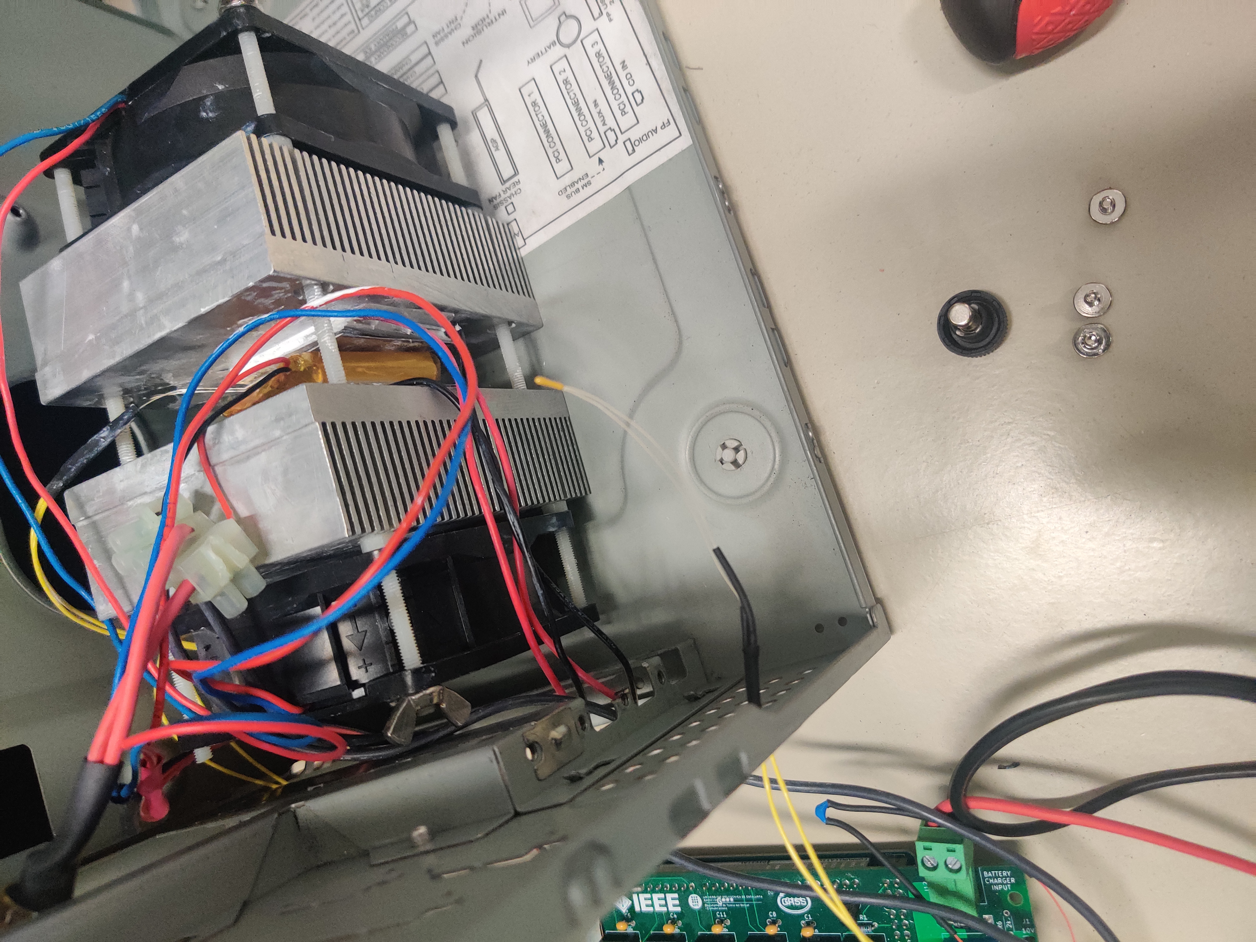
4. Place the battery between the TEC module assembly halves.

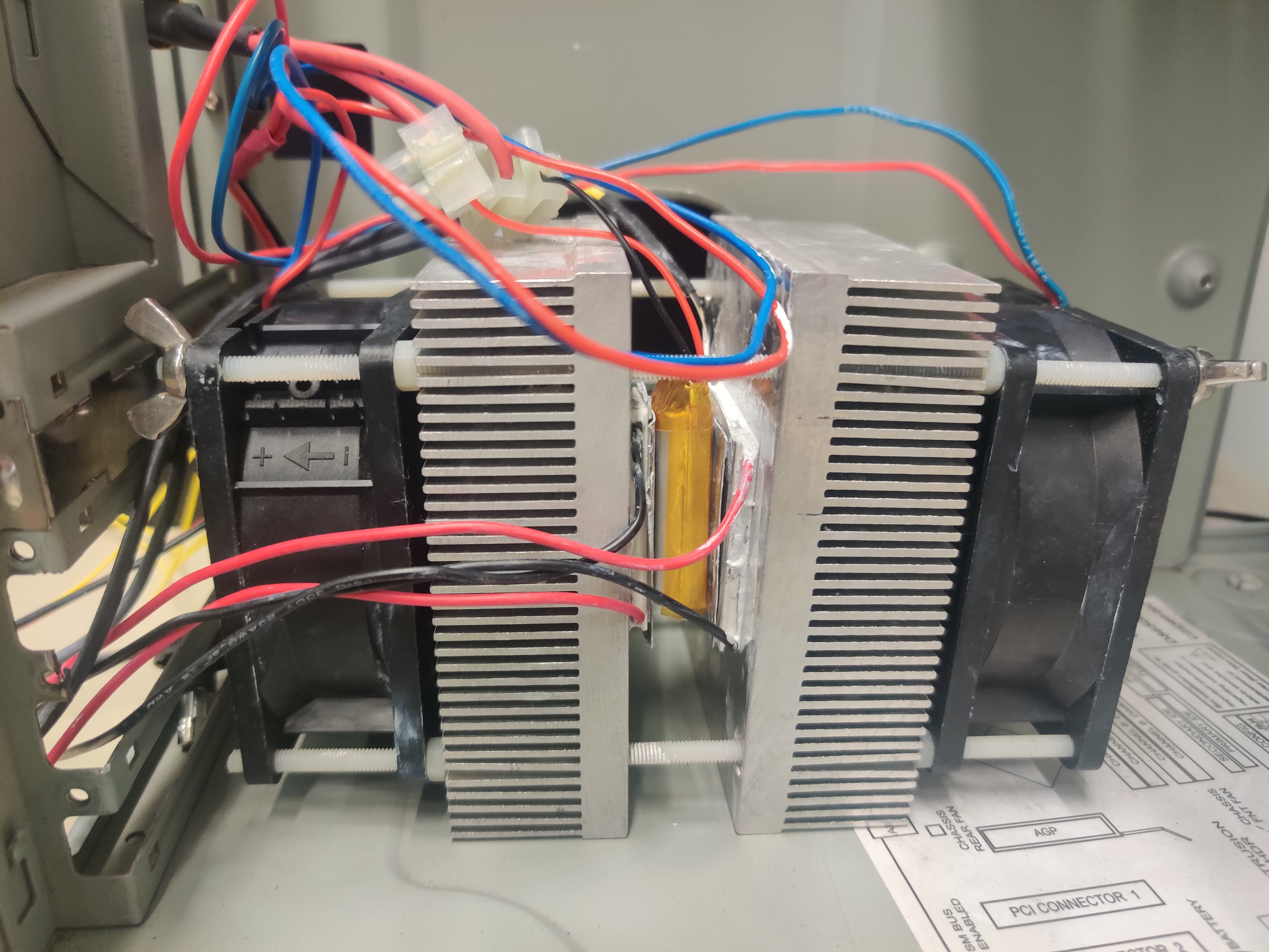
5. Place the assembly with the battery inside a metal box for protection and route the cables outside.

6. Connect the NTC, FANS and TEC modules to the battery test apartus headers (check labels especially in the case of the TEC modules)

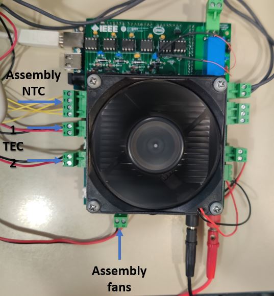
7. Conect the remaining NTC to the port labelled as NTC Heatsink and put it inside the metal box to have an ambient temperature reference point.

8. Close the metal box

9. Enable the 12V power supply output.

10. Connect the USB cable to the Arduino and PC and upload the charge .ino test code to the board. Select the adequate COM port on the Arduino IDE and remember it for the following steps.

11. Disconnect the USB cable from the PC.

12. Disable the 12V output.

13. Open PUTTY and select connection type: Serial and write down the Arduino COM port previously indentified. If the OS is Linux, it will probably be /dev/ttyACMX where 'X' is the port number.

14. In PUTTY go to the Logging tab and select Printable Output and select the folder where you want to save the test data.

15. Connect the battery cables to the terminal block labelled as BATERY respecting polarity and installing a Fuse of 2,5A between the battery test apparatus and the battery.

16. Enable both power supply channels.

17. Connect the USB cable to the PC and click on Open on the PUTTY software.

18. If all steps were performed correctly, the text START ARDUINO will be visible, and, after pressing any key of the keyboard, the test will start. Every 5 seconds a new line will be written indicating the voltage, current, accumulated power and temperature separated by a semicolon (“;”)

19. Each cycle end will be indicated on screen and at the beginning of each charge cycle the test iteration will be written. At the end of the entire test, a “TEST END” prompt will appear. Note that for a test of 10 iterations will take approximately 3 days to complete.

20. Disconnect USB cable.

21. Turn off power supplies.

22. After that the data will be available in the folder you selected before, and you can use the software you prefer to graph and analyse the result data from the CSV file.

Test Results

This battery degradation test has lasted 844 hours and taking into account that a full charge and discharge cycle lasts approximately 4 hours, a total of 211 full cycles have been performed.

1. Voltage

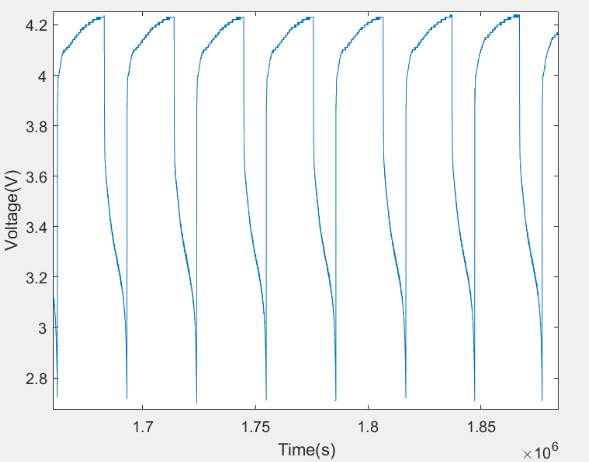
As it is seen, the votltage range is from 2.7 V to 4.3 V. It is faster for discharging than for charging because in charging mode when it is almost getting to the final charge voltage the cells are trying to get the equilibrium. For this reason, it is possible to see the slowest part from 4.1 V till 4.3 V.

2. Current

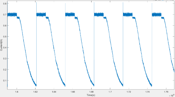
As the capacity of the battery is 1400 mAh, the current charge is 700 mA so as not to exceed the limit, for this reason we have a constant current and an almost linear discharge part as it discharges. The lowest current level is when it reaches to 2.7 V.

3. Energy

In the previous graph, the highest plots are the energy in the charge cycle and the lowest ones represents the battery discharged or provided by the battery. It is seen that the last pic compared with the first one of the lowests plots is slightly lower than the first one. Let's see the complete charge and discharge cycles of the test:

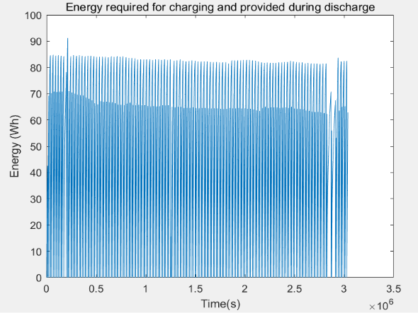
As the number of cycles increases, the battery capacity decreases. At the beggining of the test the battery provided around 70 Wh for one discharge cycle and at the end of the test it provided around 65 Wh for 1 discharge cycle.

4. Modules temperature

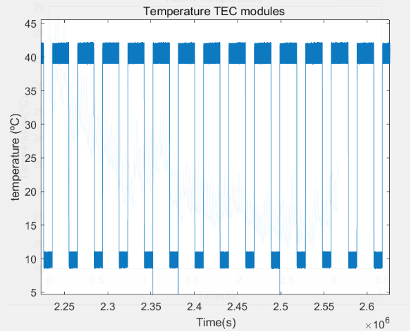
This plot represents the temperatures at the charge and discharge cycles. For charging the battery, the modules temperature is set to 40 ºC. For discharging, the temperature is set to 10 ºC.

Conclusions

It is seen in the energy plots the loss of effective energy provided by the battery. The battery starts providing 70 Wh for a discharge cycle and finally provides 65 Wh. This means that for every charge and discharge cycle is lost 23.7 mWh

On the other hand, as it can be seen in the beginning of the voltage curves, the battery was subjected to a voltage higher than the maximum due to overheating of the power sources, and there were no serious consequences for it.

Even though the test may not be entirely conclusive because of its time constraints, it does show the robustness of the battery. The PocketCube energy requirements are much smaller than the ones subjected in this test and therefore it can be concluded that the battery is suited for the mission.

The code is available at: https://github.com/nanosatlab/pocat-sw/tree/main/Battery%20test%20aparatus/Arduino%20Code/Degradation_testing

Photodiodes Temperature Characterization

Test Description and Objectives

The main objective of this test is to characterise the temperature behaviour of the photodiode and calibrate its results.

Test Set-Up

• ADCS board and the PocketQube lateral boards.
• Multimeter, alligator clips ,cables and jumpers for the connection between the photodiodes and the ADCS board.
• A computer.
• Black coated box.
  
• An halogen bulb with its correct power source.
• Hair dryer.

Test Plan

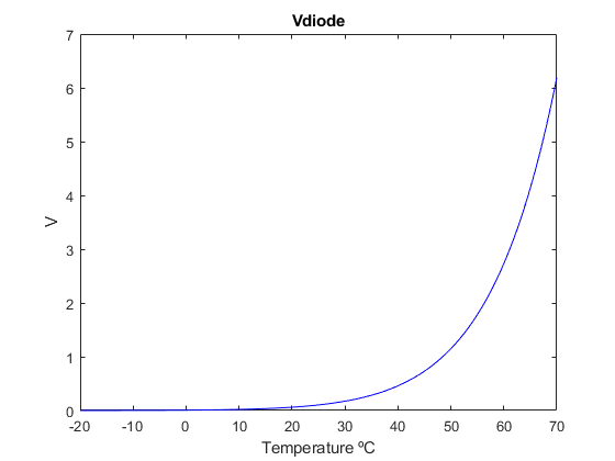
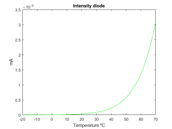
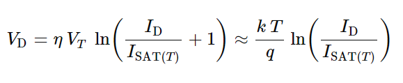
Following the Shockley Diode equation, the current coming out the photodiode depends of the temperature, following an exponential function.

The Shockley diode equation is the following one:

                                                                             

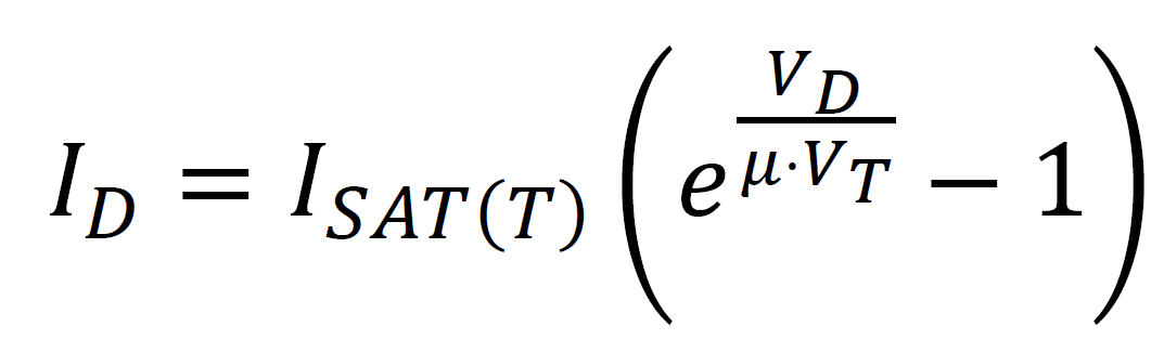
Where:

              I_D is the diode current.

              I_sat(T) is the reverse bias saturation current.

              V_D is the voltage of the diode.

              V_T is the thermal voltage.

              μ is the idiality factor, it will be assumed that it is equal to 1.

In this equation there are two key parameters, the V_T and the I_sat(T) which are computed with the following formulas:

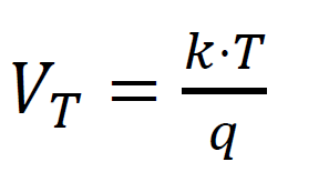
Where:

             k is the Boltzman constant in [ j/k ].

             T is the temperature of the diode in kelvins.

             q is the elementary charge.

Where:

             T_nom is the temperature in which the photodiode's characteristics are specified in the datasheet.

             E_g is the energy gap.

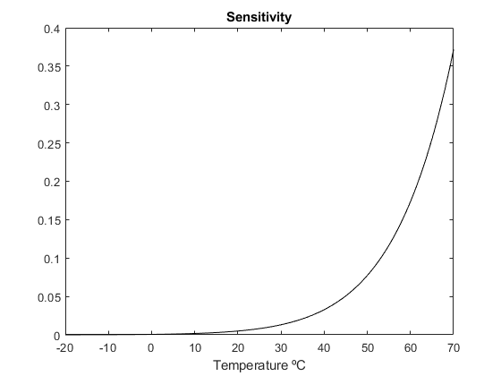
Now the next step is to derive the sensitivity equation. To obtain it, you will have to derivate the Shockley diode equation in function of the temperature:

The sensitivity in function of the temperature will have this shape:

All the parameters that  has been obtained are the following:

Computed Isat(Tnom)

Measured voltage quantized values

Measured T

At this part of the calibration the following steps have to be followed:

1. First of all, the I_sat(Tnom) has to be computed. In order to do that, you have to measure the Id and Vd of the photodiode while using a constant source of light. Afterwards, isolate the I_sat(Tnom) from the Shockley diode equation and compute it.
2. Afterwards, put the photodiode inside the black coated box pointing towards an halogen lamp bulb. You have to take measurements of the photodiode and its operating temperature. Place the box in a place where it can reach as low temperatures as you can. While the photodiode is taking measurements, the halogen lamp will increment the temperature inside the black coated box. The temperature will increase until a maximum point, then is the turn of the dryer, start increasing the temperature inside the box pintroducing hot air little by little.
3. Once the measurements are completed, the real voltage measured in the ADC can be computed, knowing that a 12-bit quantization is used.
   
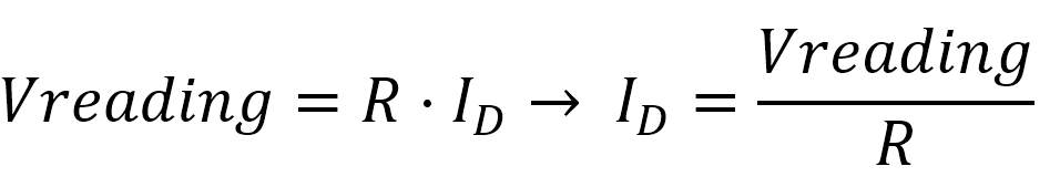
4. Next, compute the current IdI_dId​, considering that a resistor of 20 kΩ is being used.
   
5. Later, compute the Vd isolating it from the Id equation:
6. Afterwards, compute the sensitivity for each measurement using the sensivity equation. THe Vd and the temperature will be different for each measurement.
7. The last step is to calibrate the measurements using the following equation:

Test Results

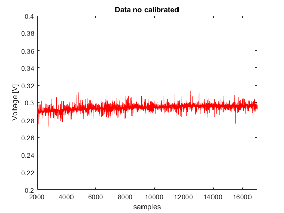
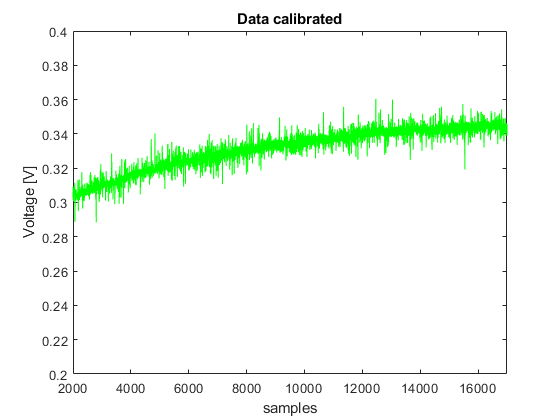
A simulation was conducted with a total of 17,000 samples of photodiode measurements taken at temperatures ranging from 15 to 35 degrees Celsius. As shown in the calibrated data, photodiode measurements increase with rising temperatures.

Conclusions

The calibration test has been conducted succesfully.

Magnetorquer Polarisation verification

DOCUMENT SCOPE

The aim of this document is to clearly explain the procedure to verify the polarisation of the magnetorquers.

TEST 1: Electrical check

Test Description and Objectives

The aim of this test is to verify that the polarisation of the magnetorquers is the correct one.

Requirements Verification

Requirement ID	Description
TST-MAGT-01	The magnetorquers must generate a magnetic field direction in accordance with the left hand rule when current is being injected.

Test Set-Up

• Power supply.
• Two bananas.
• Outer boards boards.
• Two cables per lateral board.
• A device to measure the magnetic field ( e.g magnetometer of the mobile phone ).
• Cable stripper.
• Soldering station.

Pass/Fail Criteria

The verification will be completed if the polarisation is the same as te theoretical computed using the right hand rule.

Test Plan

1. Strip the cables at both ends.
2. Turn on the soldering station.
3. Solder one cable for each extreme of the magnetorquer. Those pins are the ADCS pin and VCC_MAG pin off the outer boards.
4. Connect the power supply.
5. Set an intensity of 16 mA.
6. Connect the bananas into the power supply.
7. Take one outer board and connect the positive banana to the ADCS pin. Afterwards, connect the negative banana to the VCC_MAG pin.
8. Turn on the device used to measure the magnetic field.
9. Turn on the output of the power supply.
10. Place in the exterior face of the board, the device. Then check that the direction of the magnetic field goes out from the center of the exterior face.
11. Turn off the output of the power supply
12. Connect the negative banana to the ADCS pin. Afterwards, connect the positive banana to the VCC_MAG pin.
13. Turn on the output of the power supply.
14. Place in the inner face of the board, the device. Then check that the direction of the magnetic field goes out from the center of the inner face.
15. Turn off the output of the power supply
16. Disconnect the power supply.

Test Results

Gyroscope Characterization and Calibration

Test Description and Objectives

This test is designed to characterize and calibrate the ADCS gyroscopes, ensuring their precise performance under various conditions. The results will give us important information to improve the system that controls the satellite’s orientation, making the system more reliable and effective.

Test Set-Up

To conduct this test, an STM32L476RG Nucleo board is utilized as a simulator for the OBC-ADCS interface. Commands are sent to the Nucleo board, which subsequently requests data from the ADCS board.

• ADCS and Breakout board
• STM32L476RG Nucleo board
• Wires
• A computer with STM32CubeIde and Ki-Cad installed
• Calculator, pen and paper, or computer with Excel
• Protoboard
• 2 Resistances of 4.7 KOhms
• Peltier cell
• Halogen lamp
• Rotating platform with motor. In case of unavailability, use something that can produce a constant rotation.
• Power supply.

Test Plan

To calibrate the gyroscope IIM 42652 we have done the following test:

3.1 Allan's variance characterization

First, the “Random walk phenomenon” of the gyroscope has to be characterized. The method will use the Allan’s variance. Once the samples of measurements has been taken, the standard deviation of the measurements will be plotted in function of the time. The results might be similar to the following ones:

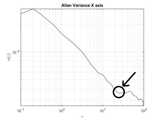
In these plots, it is observed the evolution of the standard deviation of the noise in the gyroscope samples. Approximately, in τ=10 s for the X and Z axis, and for τ=20 s, the standard variation tends to variate the slope of the line repeatedly, that happens because of the effect of the “Random walk phenomenon”.

Consequently,  the gyroscope samples will be averaged for 10 seconds, using a sample frequency of 0.1 seconds. The total number samples that will be averaged is 100 samples.

The schematic used for the averaging algorithm is the following one:

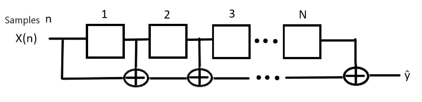
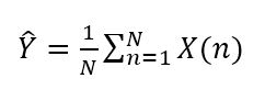
This algorithm functions as a circular queue that averages all the samples within it during each iteration, helping to reduce the effect of the "random walk phenomenon" in the gyroscope readings.

3.2 Temperature bias characterization and calibration

Afterwards, we will have to take at least 1000, or more, samples of data for each axi in differents situations using the algorithm of the previous section:

1- Static data measurements, all with a constant temperature.

• Ambient temperature, aproximately 25ºC.
• Night temperature, around 10ºC.
• Freezer temperature. around -16 ºC.
• Halogen lamp, around 40ºC.
• (optional) peltier cellwith a constant temperature different to the previous ones

2-Movement measurements

• With the rotation platform take samples of each axi in one velocity, remember to writte down the real velocity used in degrees/second and the temperature of each sample.
• With the same velocity redo the measurements now with a diferent temperature, remember to use one of the temperatures used for the previous static measurements, for example halogen lamp with 40 ºC.

After that, in order to calibrate de measurements, the following formula will be used for each axis:

                                             Data Calibrated = Data measured * sensitivity - Bias(Tº)

For each axis, plot the real data in function of the measured data using in the X axis the measured data and in the Y axis the real data. Afterwards, in the measured data vector use the static data and the constant velocity data, both obtained with the same temperature. Regarding the real data, also use the static real data and the real angular velocity data. Now you will have two figures, each one with different temperature, compute in both plots the line equation of the graphic and store the value of the slope coefficient of the equation.

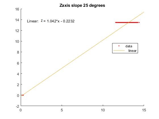
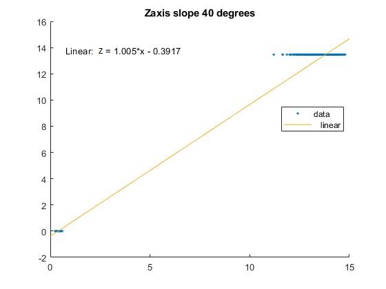
After obtaining the two slopes, one for the first temperature and the other for the second, the next step is to plot the slope, which is computed using the two previous calculated slopes, against the temperature and recalculate the line equation. This line equation will serve as the formula for calculating sensitivity as a function of temperature.

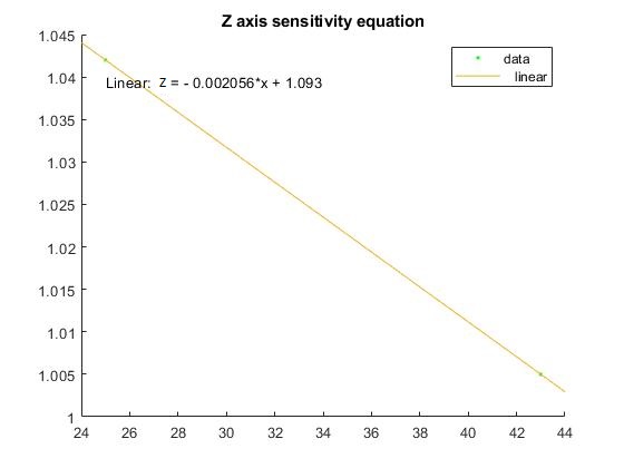
This procedure is repeated for each axis:

Axis	Slope (25 ºC)	Slope (40 ºC)	Sensitivity equation
X	1.073	1.085	Xsens=-0.0009231*T(ºC)+1.05
Y	1.026	0.9912	Ysens=-0.0029*T(ºC)+1.099
Z	1.042	1.005	Zsens=0.002056*T(ºC)+1.093

For the next step of the calibration, the measured static data versus the temperature is plotted. This graphic will show us the evolution of the bias in respect to the temperature. Then, the equation of the line will be computed, which will be used in order to compute the Bias:

            Bias( Tº) = m *  Tº(temperature) + n

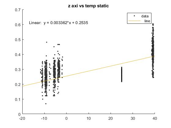
The results for each axis are:

Axies	Bias equation
X	Bias=0.01388 * T(ºC)-0.1716
Y	Bias=0.0005596 * T(ºC)-0.03862
Z	Bias=0.003362 * T(ºC)+0.2535

The final calibrated data will be computed with the following equation:

Calibrated_data = Sensitivity(ºC) * Measured_data - Bias(ºC)

Test Results

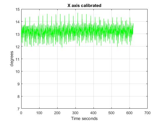
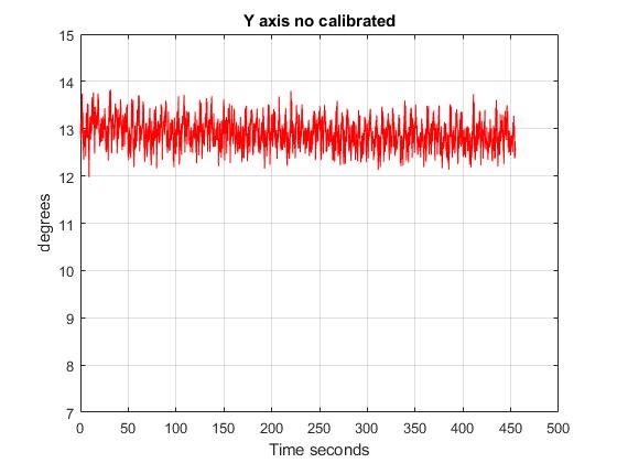
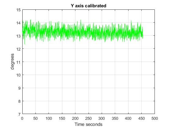
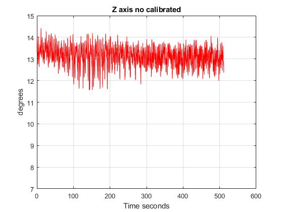
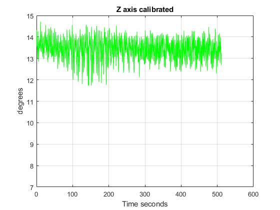
The test consisted of measurements of a real velocity of 13,6 degrees/s. The following plots show that the results of the calibration in all the axis.

                             

                             

                           

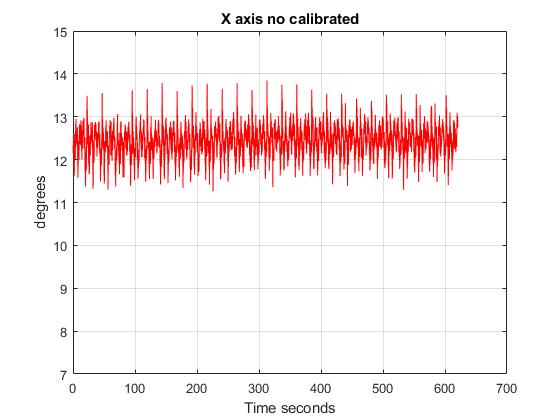
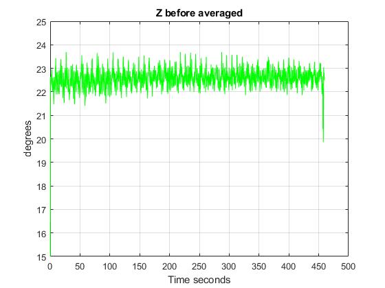
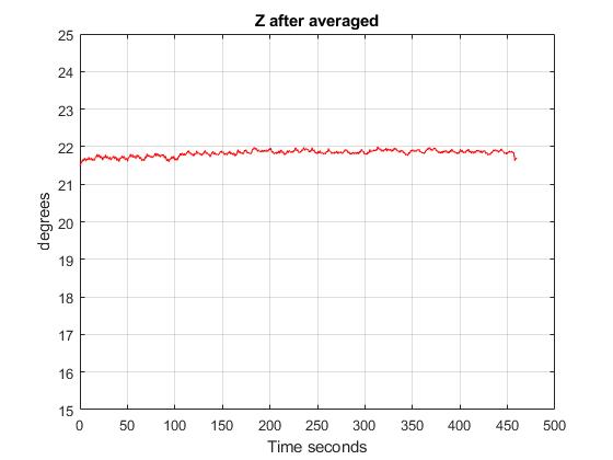
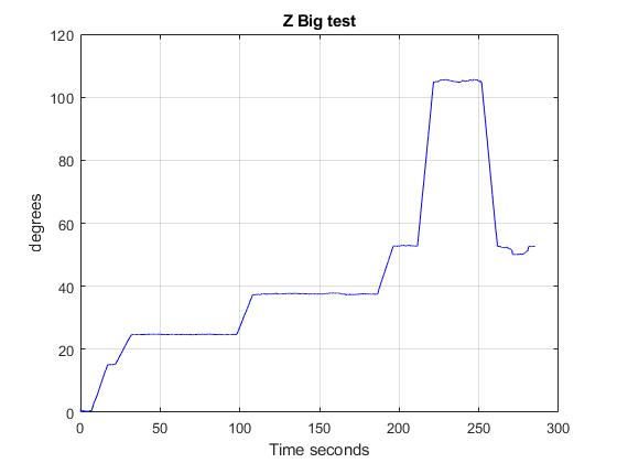
In addition, the following figures show the results of testing the averaged algorithm. The tests show how the gyroscope works once it has been calibrated. To do so, different velocities had been applied into the Z axis. Here are the results:

                       

         

Anomalies

The temperature sensor inside the IIM 42652 could work wrongly if the chip has been exposed to high temperatures during the welding process. It is recommendable to check in the IIM 42652 documentation, which is the maximum temperature that the temperature sensor can withstand without getting damaged.

Conclusions

As all the requirements has been fulfilled, the test is completed.