# Link and Data Budget Analysis # Link budget ## Introduction A link budget assesses the various gains and losses that impact signal transmission from the satellite to the ground station, ensuring the communication link meets performance requirements. By analyzing key factors such as transmission power, antenna gains, path losses, and atmospheric attenuation, we predict the signal-to-noise ratio (SNR) and system reliability. This revised document details the methodology, assumptions, and calculated outcomes, providing a comprehensive understanding of the system’s performance and limitations. These results are essential for validating the design and ensuring reliable data transmission for the IEEE Open PocketQube Kit mission. Please check the [data budget](https://wiki.nanosatlab.space/books/cat-mission-analysis-and-characterisations/page/data-budget "Data budget") for additional information regarding COMMS budgets. ## Methodology The methodology for calculating the link budget involves several key steps. First, we generated separate tables for each type of link: uplink and downlink. For each link, three different scenarios were considered: nominal, adverse, and favorable. - Nominal scenario: Normal operation and conditions. - Adverse scenario: Worst expected performance. - Favorable scenario: Best possible performance. It is important to note that all scenarios are calculated at a fixed orbit altitude of 500 km. The adverse and favorable scenarios have been updated to assess the variability of other parameters, such as antenna gain and losses. Additionally, we have revised the valid link margin for the nominal scenario to 3 dB for an orbit altitude of 500 km. Finally, calculations for the −3σ and RSS worst case have been performed using the adverse and favorable scenarios.

Parameter	Value	Description
Central Frequency \[MHz\]	868
Bandwidth \[kHz\]	125
Spreading Factor	11
Orbit Height \[km\]	500	Fixed altitude as per the Mission Analysis calculations.
Maximum Transmitted Power \[dBm\]	22	Maximum transmitted power as specified in the transceiver datasheet (SX1262).
Gain of the Monopole Antenna \[dBi\]	4	A quarter-wavelength monopole antenna has a gain of 5.15 dB. To account for a safety margin, we assume a gain of 4 dBi for the antenna.
Gain of the Patch Antenna \[dBi\]	12	Gain of the GS Yagi antenna as specified in the datasheet.
Polarization Losses \[dB\]	3	3 dB as we are using circular polarization.
Losses Due to Atmosphere \[dB\]	2	According to ITU-R recommendation 618, atmospheric losses are very small, primarily due to ionospheric scintillation. Also, ITU-R P.840-8 shows negligible attenuation due to clouds and rain at 868 MHz. Atmospheric losses are considered to be 2 dB.
Losses Safety Margin \[dB\]	3	As recommended in one of the RIDs, a link margin of 3 dB is applied.
Sensitivity for SF=11 \[dBm\]	-134.5	Given our bandwidth and spreading factor, our sensitivity is -134.5 dBm.
Sensitivity for SF=11 \[dB\]	-17.5	SNR sensitivity is -17.5 dB.

Please note that the gain of the quarter-wavelength monopole antenna shown in the table is 4 dBi. The theoretical gain of a quarter-wavelength monopole antenna is based on the gain of a half-wave dipole antenna, which is approximately: [![image.png](https://wiki.nanosatlab.space/uploads/images/gallery/2024-10/scaled-1680-/OcOimage.png)](https://wiki.nanosatlab.space/uploads/images/gallery/2024-10/OcOimage.png) Since a quarter-wavelength monopole antenna radiates only over half of the space due to the presence of a ground plane, its gain increases by 3 dB. Therefore, the gain of the monopole antenna is given by: [![image.png](https://wiki.nanosatlab.space/uploads/images/gallery/2024-10/scaled-1680-/TC7image.png)](https://wiki.nanosatlab.space/uploads/images/gallery/2024-10/TC7image.png) To incorporate a safety margin in our calculations, we assume a gain of 4 dBi for the quarter-wavelength monopole antenna. ## Study cases This section introduces each one of the scenarios that will be used for this link budget.

Favorable Scenario	Nominal Scenario	Adverse Scenario
500 km orbit height	500 km orbit height	500 km orbit height
0dB pointing losses	0.5dB pointing losses	1dB pointing losses
5.15dBi antenna gain	4dBi antenna gain	0dBi antenna gain (no deployment)
3dB link margin	3dB link margin	3dB link margin

## Analysis of the results This section presents the results from the Link budget analysis, detailing the findings for each study case across all three scenarios. ### Power and SNR requirements After running the code we created to compute the link budget, we have generated Figures shown below. These figures display the received powers for both Downlink and Uplink at each edge, as well as the corresponding SNR values. Note that the sensitivities outlined in the previous section are also represented as lines in the plots. The analysis of these results will determine the **minimum elevation angle** **required for contact**, identified by the intersections between the thresholds and the received power or SNR. A summary of the results is presented in this table:

Scenario	Favorable		Nominal		Adverse
	Prx	SNR	Prx	SNR	Prx	SNR
Downlink \[min elevation angle\]	0	0	4	0	17	1
Uplink \[min elevation angle\]	0	0	0	0	5	0

[![image.png](https://wiki.nanosatlab.space/uploads/images/gallery/2024-10/scaled-1680-/FKoimage.png)](https://wiki.nanosatlab.space/uploads/images/gallery/2024-10/FKoimage.png) [![image.png](https://wiki.nanosatlab.space/uploads/images/gallery/2024-10/scaled-1680-/CTgimage.png)](https://wiki.nanosatlab.space/uploads/images/gallery/2024-10/CTgimage.png) [![image.png](https://wiki.nanosatlab.space/uploads/images/gallery/2024-10/scaled-1680-/Il3image.png)](https://wiki.nanosatlab.space/uploads/images/gallery/2024-10/Il3image.png) [![image.png](https://wiki.nanosatlab.space/uploads/images/gallery/2024-10/scaled-1680-/QGoimage.png)](https://wiki.nanosatlab.space/uploads/images/gallery/2024-10/QGoimage.png) ## Conclusions Once the link was computed, we looked for the references on the LoRa to demonstrate the disability of the link despite having a negative SNR \[1\]. Also, the approach to use LoRa on our mission was due to a recommendation from our professor, as the theoretical feasibility was demonstrated in \[2\]. To conclude, in addition to some experiments, \[2\] helped us to choose SF =11 and BW = 125 kHz. 1. **Favorable Scenario:** \- Both uplink and downlink communications are highly reliable. \- Minimum elevation of 0°, ensuring robust communication links. 2. **Nominal Scenario:** \- Taking into account an antenna gain of 4dBi and a link margin of 3dB as recommended by ESA's expert. \- Communications remain reliable, though with slightly higher minimum elevation angles (4° for downlink and 0° for uplink). \- Communications are feasible but require more optimal conditions compared to the favorable scenario, especially for the downlink. 3. **Adverse Scenario:** \- Taking into account no antenna deployment as well as worst system performance. \- Uplink communication is possible but requires minimum elevation of 5°. \- Downlink communication is possible but requires minimum elevation of 17°. In our analysis, we calculated the −3σ margin, which provides a conservative estimate of the link performance under adverse conditions. The calculated −3σ margin was found to be 4.9505, indicating the minimum acceptable performance level for reliable communication. Additionally, the worst-case RSS analysis yielded a total RSS of 3.4689. This worst-case scenario confirms the robustness of our system, with a link margin superior to 0 dB, as it demonstrates the ability to maintain communication links even under challenging conditions. Both parameters were calculated as detailed in ECSS-E-ST-50-05C, section 8. The link budget analysis demonstrates the feasibility of our communication system for the PoCat Lektron mission PocketQubes, developed under ESA’s FYS4! program. The analysis considers different scenarios for uplink and downlink communications, including favorable, nominal, and adverse conditions. Moreover, when taking adverse conditions, we find that communication is possible even in challenging scenarios. This confirms the link’s feasibility. ## References \[1\] RF Wireless World. LoRa Sensitivity Calculator. [https://www.rfwireless-world.com/calculators/](https://www.rfwireless-world.com/calculators/) LoRa-Sensitivity-Calculator.html, 2024. \[2\] L. Fernandez, J. A. Ruiz-De-Azua, A. Calveras, and A. Camps. Assessing lora for satellite-to-earth communications considering the impact of ionospheric scintillation. IEEE Access, 8:165570–165582, 2020. # Data budget

Introduction

This document outlines the methodology, assumptions, and calculated results, providing a clear understanding of the system’s data management and limitations. These results are crucial for validating the design and ensuring reliable data transmission for the IEEE Open PocketQube Kit. Please check the link budget for additional information regarding COMMS budgets.

Methodology

As detailed in the link budget, the simulated nominal scenario for obtaining values and performing computations involves an orbital height of 500 km.

To determine the data budget, we need to calculate the maximum amount of data that can be downloaded in a single pass. This requires computing the capacity for a Spreading Factor (SF) of 11 and a Code Rate (CR) of 4/5. Using the formulation provided in [1], we obtain a rate of 537.11 bps.

After obtaining the data rate, we propagated the orbits using Orbitron [2] to study the initial scenario. This software has an inclination error of 0.1º. The propagation results provided the satellite passes over the Ground Station (GS) at Montsec [3], factoring in the minimum elevation angle. Using the simulated pass durations and the calculated data rate, we calculated the data that can be transmitted during each pass over our ground station.

We then compared the average data that can be transmitted in uplink and downlink with the required data for sending commands from the satellite and the GS. We verified that the available data was sufficient to transmit and receive telecommands and payload results, and ensured that data could be re-sent if needed, as there are no protocols guaranteeing packet reception.

The table below estimates the total data volume needed for transmission during each satellite pass, covering both telemetry/configuration data and payload data for a single measurement.

Downlink
Telemetry data	48 Bytes
Configuration data	32 Bytes
Payload 1 (L band) data	2831 Bytes
Payload 2 (K band) data	708 Bytes

This data will be stored inside the satellite with up to 1MByte of storage. For the uplink, we have a variety of telecommands available.

A detailed list of all telecommands, along with the corresponding telemetry, can be found here.

Since the number of bytes required for the uplink will largely depend on the amount of available platform data and the satellite’s latest status, estimating the exact byte count for the uplink is impractical.

However, as indicated in the summary table, the PocketQubes will have a large margin, ensuring that even in a worst-case scenario—where a significant number of commands need to be uploaded during a pass—there will be sufficient time to do so.

Results

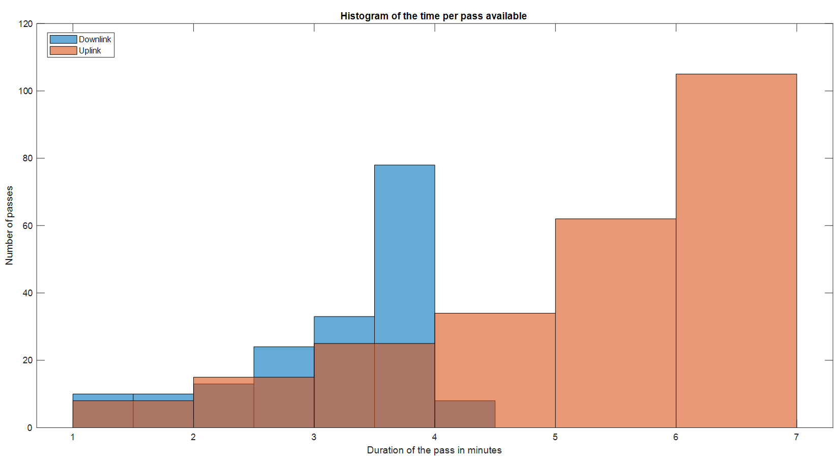
This section presents the results from the Data budget analysis. First, we have computed the number of passes available with its corresponding duration. Figure below shows the number of passes according to its duration for both uplink and downlink in 100 days:

After obtaining the results from Figure G.5, we can compute the data that can be sent during each pass based on the findings presented in [1]. On average, we have 2.49 uplink passes per day over a period of 100 days. For the downlink, we achieve about 1.63 passes per day. Table below presents the results, showing the average duration of the passes for both uplink and downlink.

Average pass time [min]
Uplink	5.26
Downlink	3.18

The data was obtained by multiplying the rate by the time per contact, resulting in the outcomes shown in the Figure below. This figure displays the amount of data available for download per pass, revealing the number of contacts related to the downloaded data. To summarize the findings from the Figure below, tables are provided, offering an overview of the average data downloaded per pass using the results from the Table above. The presented results indicate the data downloaded per pass and per day.

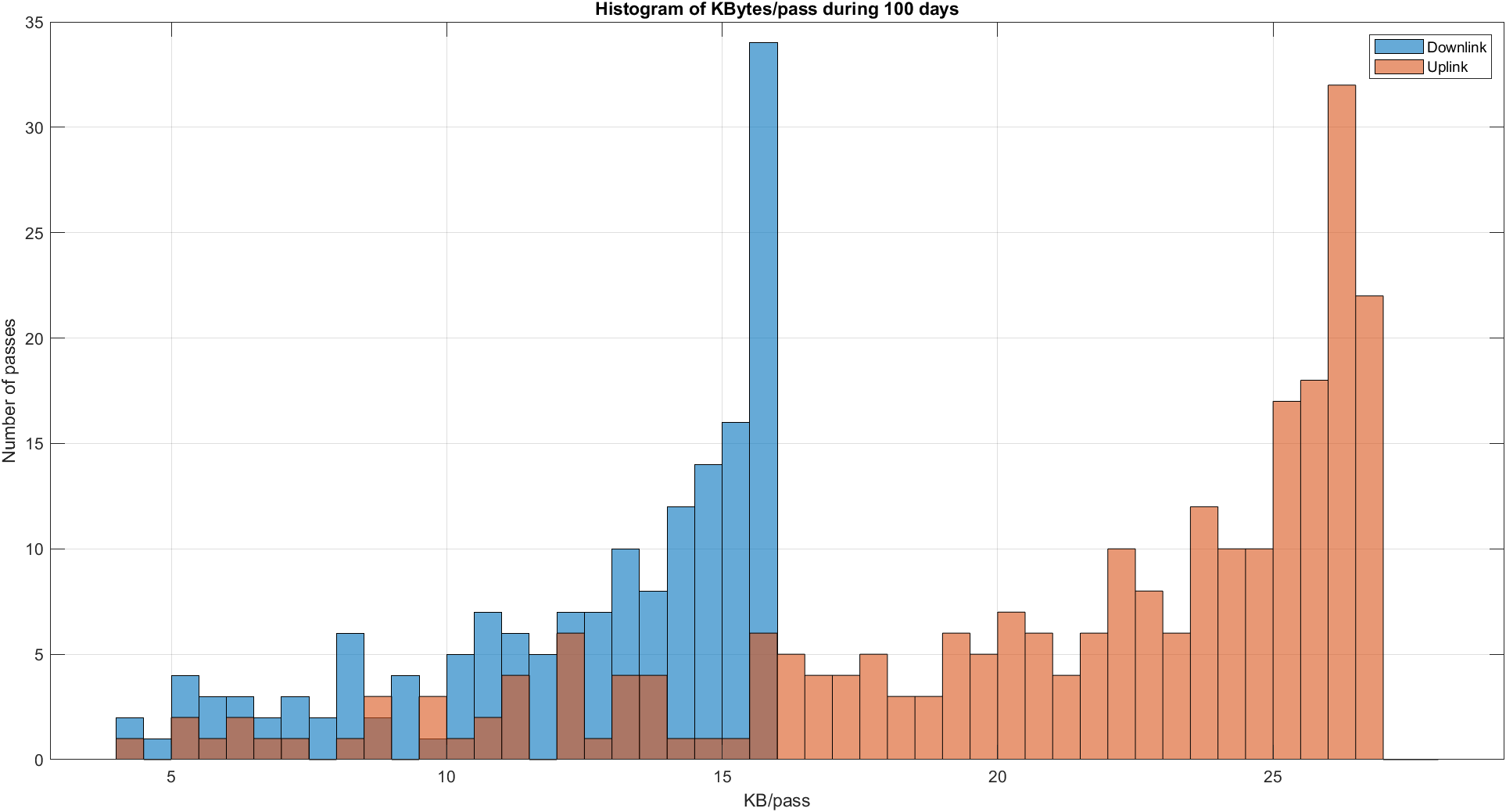
Average transmitted Bytes per pass [kBytes]
Uplink	20.69
Downlink	12.52

Average transmitted Bytes per day [kBytes]
Uplink	52.05
Downlink	22.26

From the results in the Tables above, we can now gauge the link’s capabilities for downloading data. Lastly, Figure below illustrates the kBytes per pass in relation to the maximum elevation angle the satellite reaches during that pass, which directly correlates with the maximum data we can download.

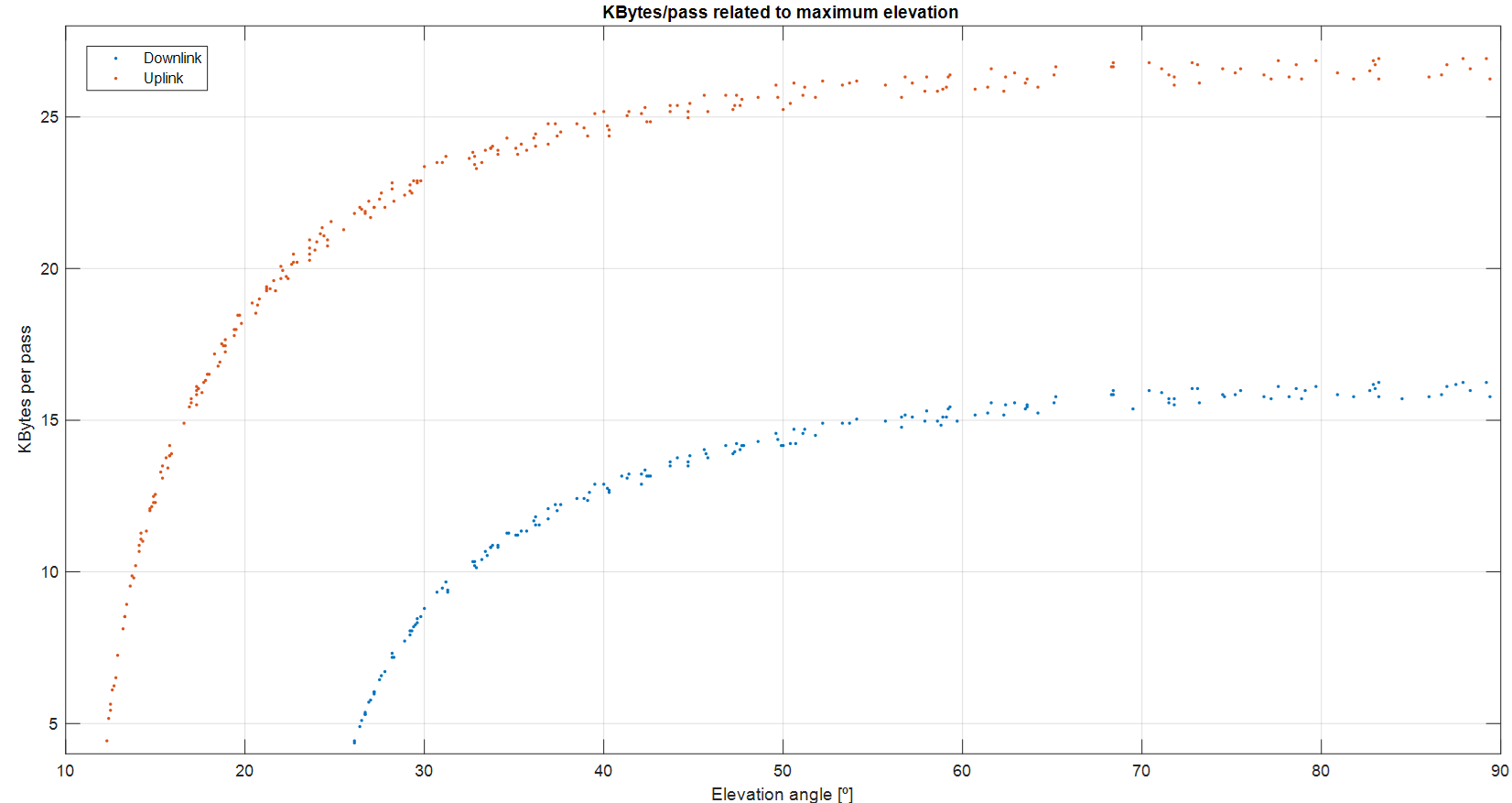
Analyzing the results, we find that the uplink transmission capacity is 20.69 kBytes. For the downlink case, the transmission capacity is 12.52 kBytes, while the L-band payload (which is the payload generating more data) requires 2831 Bytes (2.76 kBytes) to be downloaded from the satellite to the ground station. Therefore, we can conclude that the data budget capabilities are sufficient and that additional stored data could also be transmitted from the satellite to the ground station.

Conclusions

Table below demonstrates our capability to transmit at least one image per contact. Additionally, telemetry data can be sent along with the image once per pass. Furthermore, we have the ability to repeat messages if necessary to ensure successful transmission.

	Maximum Data Volume capability per pass [Bytes]	Estimated Data Volume to be transmitted [Bytes]	Additional available Bytes	Feasibility
Uplink	21191	x	20567	TRUE
Downlink PL1	12824	2831	9993	TRUE
Downlink PL2	12824	708	12116	TRUE

Additionally, following the recommendation of ESA’s expert, we present a demonstration of the data budget’s feasibility, factoring in the time required to transmit all the data. Specifically, the airtime for each packet will be approximately 1478 ms [4].

By adding a few seconds for computation time and a margin of error and considering an average pass, we arrive at:

	Data to be transmitted [Bytes]	Time required to transmit data [s]	Time left [s]	Feasibility
Uplink	500*	18.5 (+2) = 20.5	295.1	TRUE
Downlink PL1	2873	106.2 (+2) = 108.2	82.6	TRUE
Downlink PL2	708	26.2 (+2) = 28.2	162.6	TRUE

It can be observed that both PocketQubes will have sufficient time to communicate and transmit all the necessary data to the ground station, confirming the feasibility of this data budget.

* It is important to note that for the uplink, we have selected a data size of 500 bytes for transmission. As mentioned earlier, the exact amount of data required for the uplink will depend on various factors.

References

[1] RF Wireless World. LoRa Sensitivity Calculator. https://www.rfwireless-world.com/calculators/ LoRa-Sensitivity-Calculator.html, 2024.

[2] Stoff Industries. Orbitron - Satellite Tracking System - Official Website. https://www.stoff.pl/ , 2024.

[3] Parc Astronòmic Montsec. Parc Astronòmic Montsec. https://parcastronomic.cat/es/ , 2024

[4] The Things Network. The things network airtime calculator. Online Tool, 2024.

Scenario	Favorable		Nominal		Adverse
	Prx	SNR	Prx	SNR	Prx	SNR
Downlink \[min elevation angle\]	0	0	4	0	17	1
Uplink \[min elevation angle\]	0	0	0	0	5	0