Datasheet and 3D model of our Ligtricity s3040_CIC solar cell https://satsearch.co/products/exa-solar-cells-30-40
This page states that it belongs to another company ‘Ecuadorian Space Agency (EXA)’ but the datasheet and 3D model correspond to the solar cell used in this Kit.
The objective of this test is to perform and analyse a charge cycle of the battery using the battery test equipment.
| Requirement | Description |
|---|---|
| 1 | Battery can be completely charged |
| 2 | Battery can be completely discharged |
| 3 | Battery voltage shall be recorded during all the test duration |
| 4 | Battery current shall be recorded during all the test duration |
| 5 | Battery temperature shall be recorded during all the test duration |
| 6 | Total power charged to the battery shall be recorded |
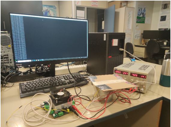
The test setup can be seen below
This test is designed to characterize a charge cycle for the PocketQube battery. There is no pass or fail criteria as the result will be the charge curves of the battery. However, after having these curves, depending on the application, further study can be needed, in order to determine whether the battery is suitable for the desired task.

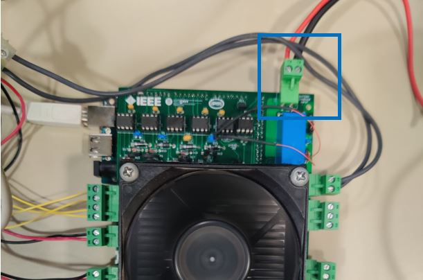
Attach the NTC to the battery under test using tape. Wrap it as tight as possible to ensure good contact between the NTC and the battery. The NTC that needs to be attached to the battery is the TOP one from NTC Battery 4 pin block terminal marked with a yellow dot on the block terminal.
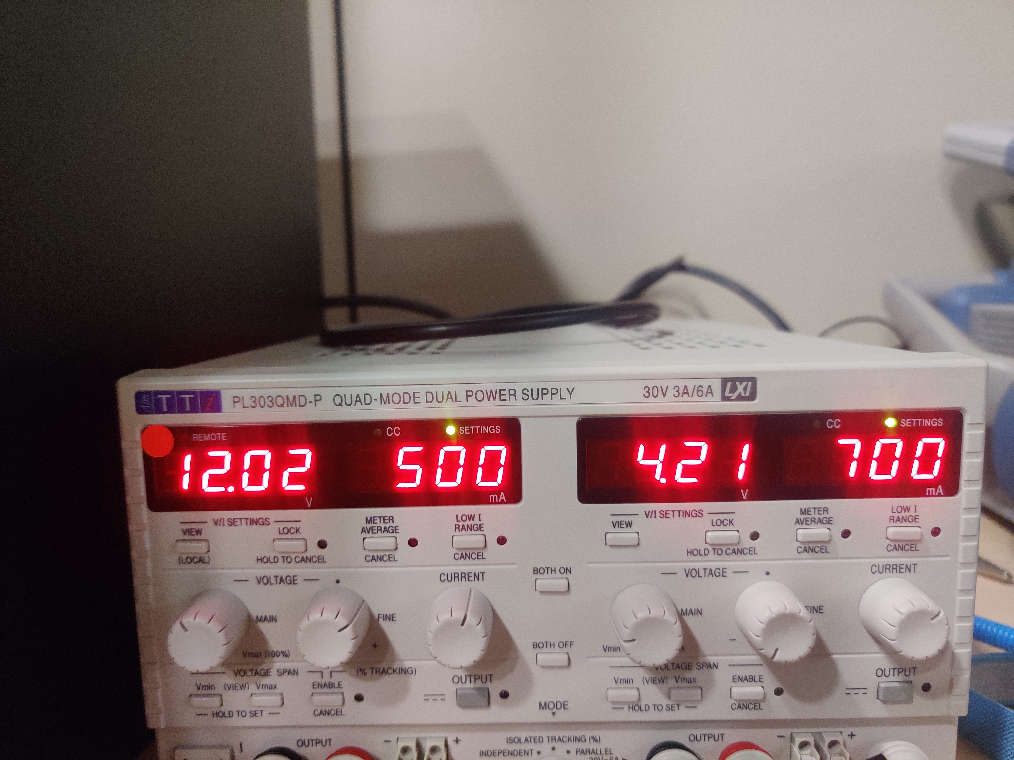
Enable the 12V power supply output.
Connect the USB cable to the Arduino and PC and upload the charge .ino test code to the board. Select the adequate COM port on the Arduino IDE and remember it for the following steps.

Disconnect the USB cable from the PC.
Disable the 12V output.
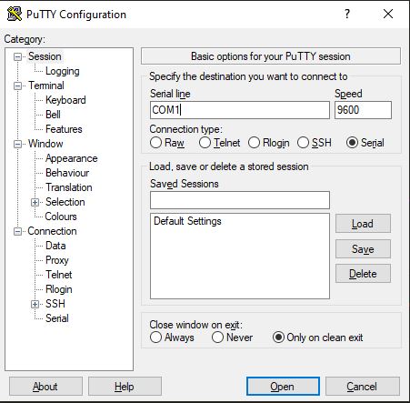
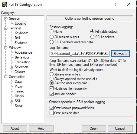
Open PUTTY and select connection type: Serial and write down the Arduino COM port previously indentified.
Put the battery inside the metal container as a precaution measure in case of explosion.
Enable both power supply channels.
Connect the USB cable to the PC and click on Open on the PUTTY software.
If all steps were performed correctly, the text START ARDUINO will be visible, and, after pressing any key of the keyboard, the test will start. Every 5 seconds a new line will be written indicating the voltage, current, accumulated power and temperature separated by a semicolon (“;”).
Each cycle end will be indicated on screen and at the beginning of each charge cycle the test iteration will be written. At the end of the entire test, a “TEST END” prompt will appear. Note that for a test of 10 iterations will take approximately 3 days to complete.
Disconnect USB cable.
Turn off power supplies.
After that the data will be available in the folder you selected before, and you can use any software capable to graph and analyse the result data from the CSV file.
This test was carried out at NanosatLab between 02/06/2023 and 05/06/2023 by Adrià Molló Carulla. The RAW data in CSV and also the processed data in an Excel file is attached to this document. This has been performed at ambient temperature (cca 25C). While already a good breakthrough, if time allows, a hot (40C) and cold (4C) case should also be performed for at least 5 cycles.
Frome the test the following results have been obtained:
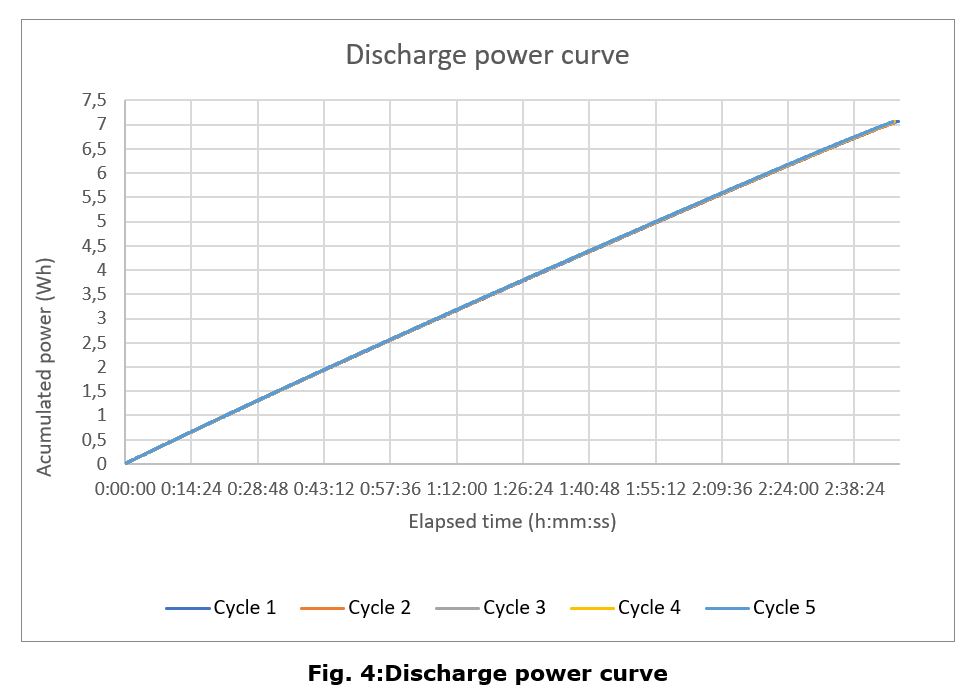

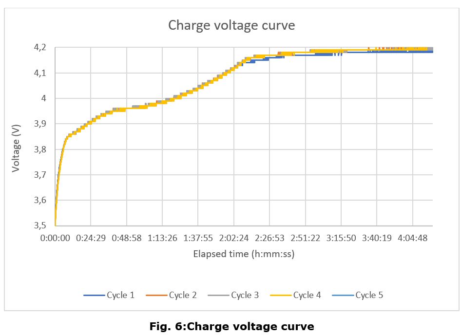
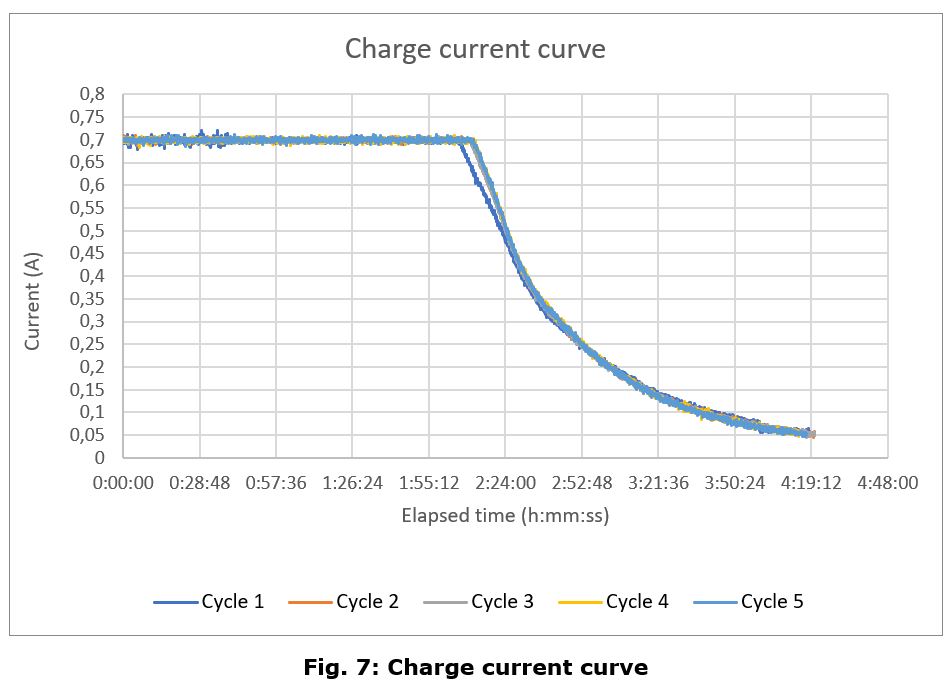
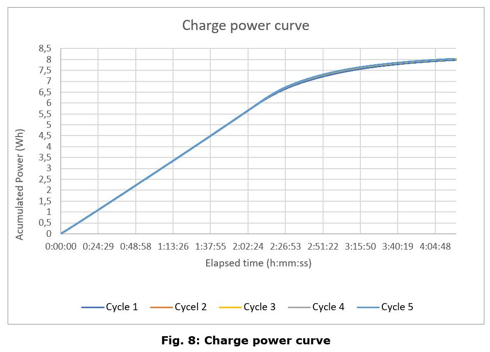
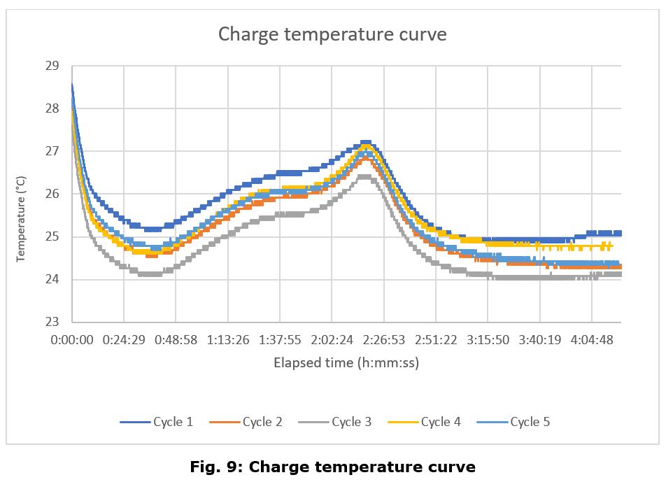
In Table 1 there is an overview of the main parameters of the battery for each iteration 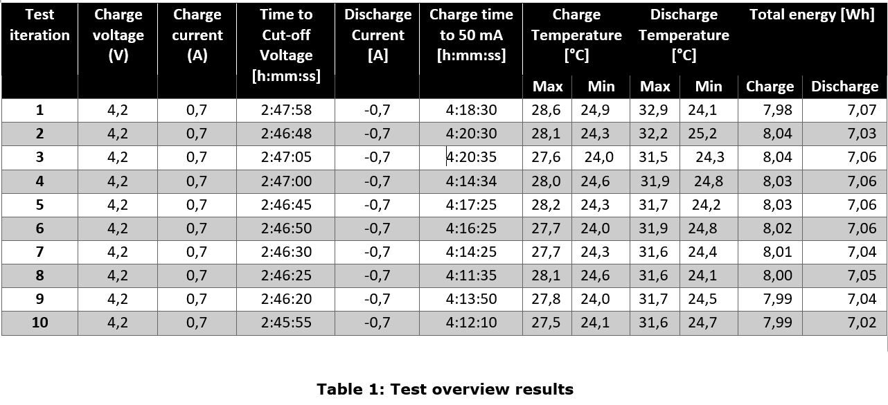
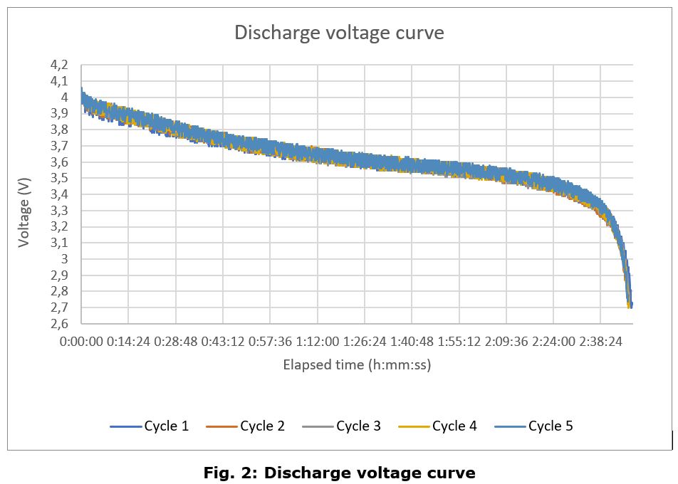
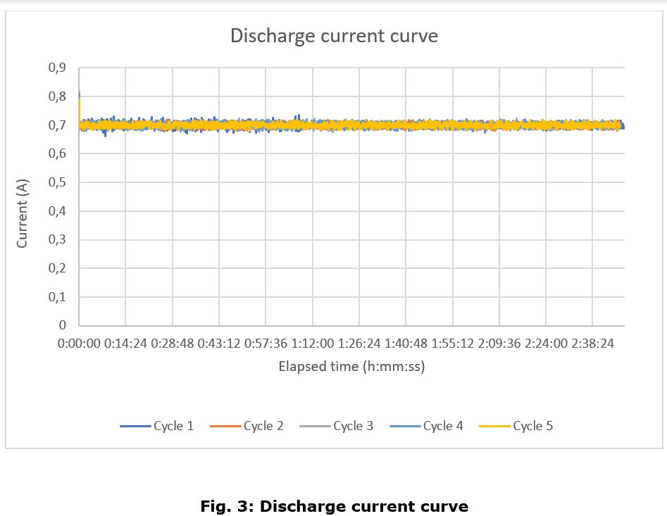
It has been found that the battery capacity appears to be considerably higher than the declared by the manufacturer (5,16 Wh) compared to the tested one (7,07 Wh).
The main conclusions of this test campaign are that the battery charge and discharge curves look follow the same pattern as a generic lithium polymer battery, with no appreciable differences, except for the aforementioned anomaly.
The full test code is available at:
Link broken, to be inserted.
# Battery degradation test ## Test Description and Objectives The objective of this test is to perform and analyse the degradation of the battery in LEO orbit thermal conditions. Due to time constraints, in order to see the proper degradation of the battery, a full charge and discharge of the battery will be carried out. That is, charging to 4.2V and discharging till 2.7V at a rate of C/2 mA. As to the temperature conditions, the same logic has been followed. The charging cycle will be done at the highest possible working temperature (40ºC) and a moderate 10ºC for the discharge cycle (instead of the lowest 2ºC). This configuration has been adopted because the battery will normally be charged by the solar panels when the PocketCube is facing the sun and discharged during the eclipse phase. ## Requirements Verification | Requirement ID | Description | | - | - | | 1|Battery can be charged | | 2 |Battery can be discharged | | 3| Battery voltage shall be recorded during all the test duration | | 4 |Battery current shall be recorded during all the test duration | | 5| Battery temperature shall be recorded during all the test duration | | 6| Total power charged to the battery shall be recorded | | 7| LEO thermal conditions must be simulated | ## Test Set-Up - Subsystem and its components. - Battery tests apparatus. - 2 power supply cables with bananas in both sides. - 2 power supply cables with bananas in one side and exposed copper in the other one. - Dual power supply or 2 independent ones. One must be able to supply 12V and 6A the other one must be able to supply 4,2V and 1A. - Flat small screwdriver. - USB A to USB B cable. - Computer with the Arduino IDE and Putty Installed to log data. - Battery to perform the test one. - 2,5 A Fuse and fuse holder. - Some wire. - Connectors to connect cable between them. - Empty metal case for the battery. ## Pass/Fail Criteria This test is designed to characterize a degradation of the PocketQube battery over a great number of cycles and temperature ranges. There is no pass or fail criteria as the result will be the information pertaining to the charge and discharge curves of the battery. ## Test Plan 1. Regulate the power supply with one channel set to 12V and 6 A and the other channel set to 4,2V and adjust the current limit so it matches the max desired charge current. [](https://wiki.nanosatlab.space/uploads/images/gallery/2023-06/img-20230621-164811.jpg) 2. Connect with 2 banana cables the 12V output from the power supply to the banana connectors from the battery test apparatus respecting the polarity. DO NOT ENABLE THE POWER SUPLY OUTPUT YET. [](https://wiki.nanosatlab.space/uploads/images/gallery/2023-06/MUGcaptura.JPG) 3. Connect the output from the 4,2V power supply to the top terminal block labelled as BATTERY CHARGE INPUT respecting the polarity. DO NOT ENABLE THE POWER SUPLY OUTPUT YET. [](https://wiki.nanosatlab.space/uploads/images/gallery/2023-06/captura2.JPG) 4. Place the battery between the TEC module assembly halves. [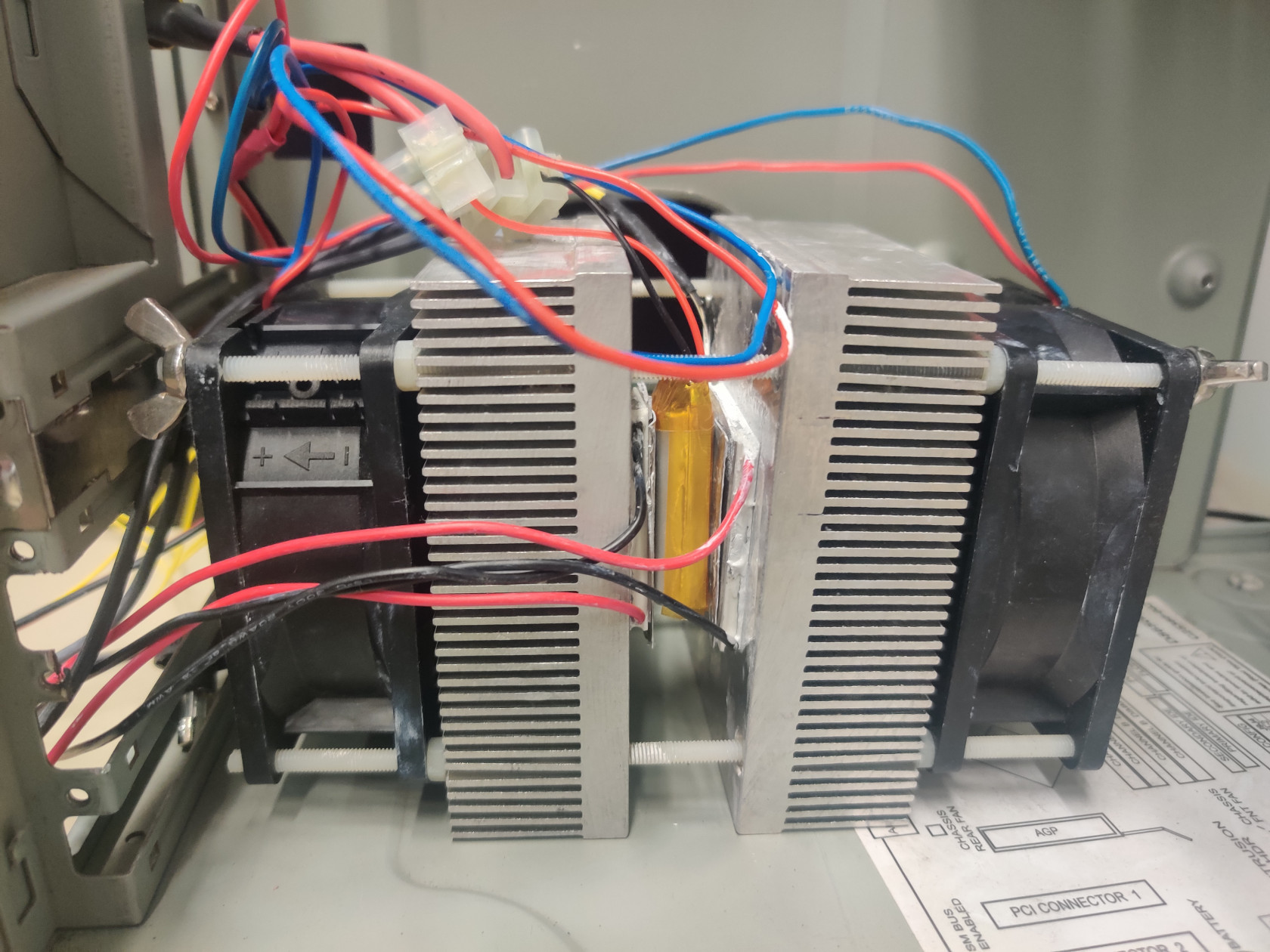](https://wiki.nanosatlab.space/uploads/images/gallery/2023-06/img-20230621-162240.jpg) 5. Place the assembly with the battery inside a metal box for protection and route the cables outside. [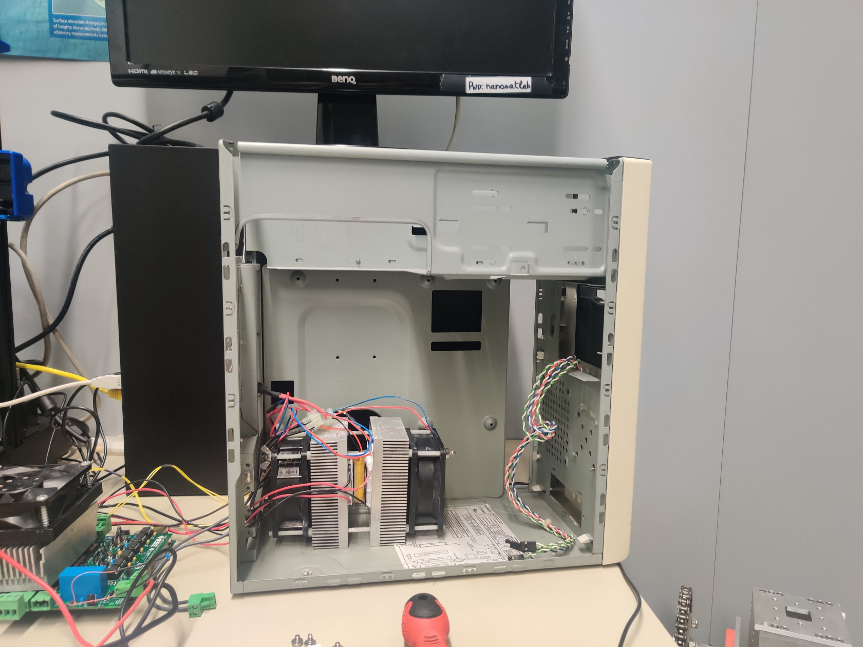](https://wiki.nanosatlab.space/uploads/images/gallery/2023-06/img-20230621-162246.jpg) 6. Connect the NTC, FANS and TEC modules to the battery test apartus headers (check labels especially in the case of the TEC modules) [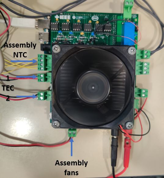](https://wiki.nanosatlab.space/uploads/images/gallery/2023-06/captura10.JPG) 7. Conect the remaining NTC to the port labelled as NTC Heatsink and put it inside the metal box to have an ambient temperature reference point. [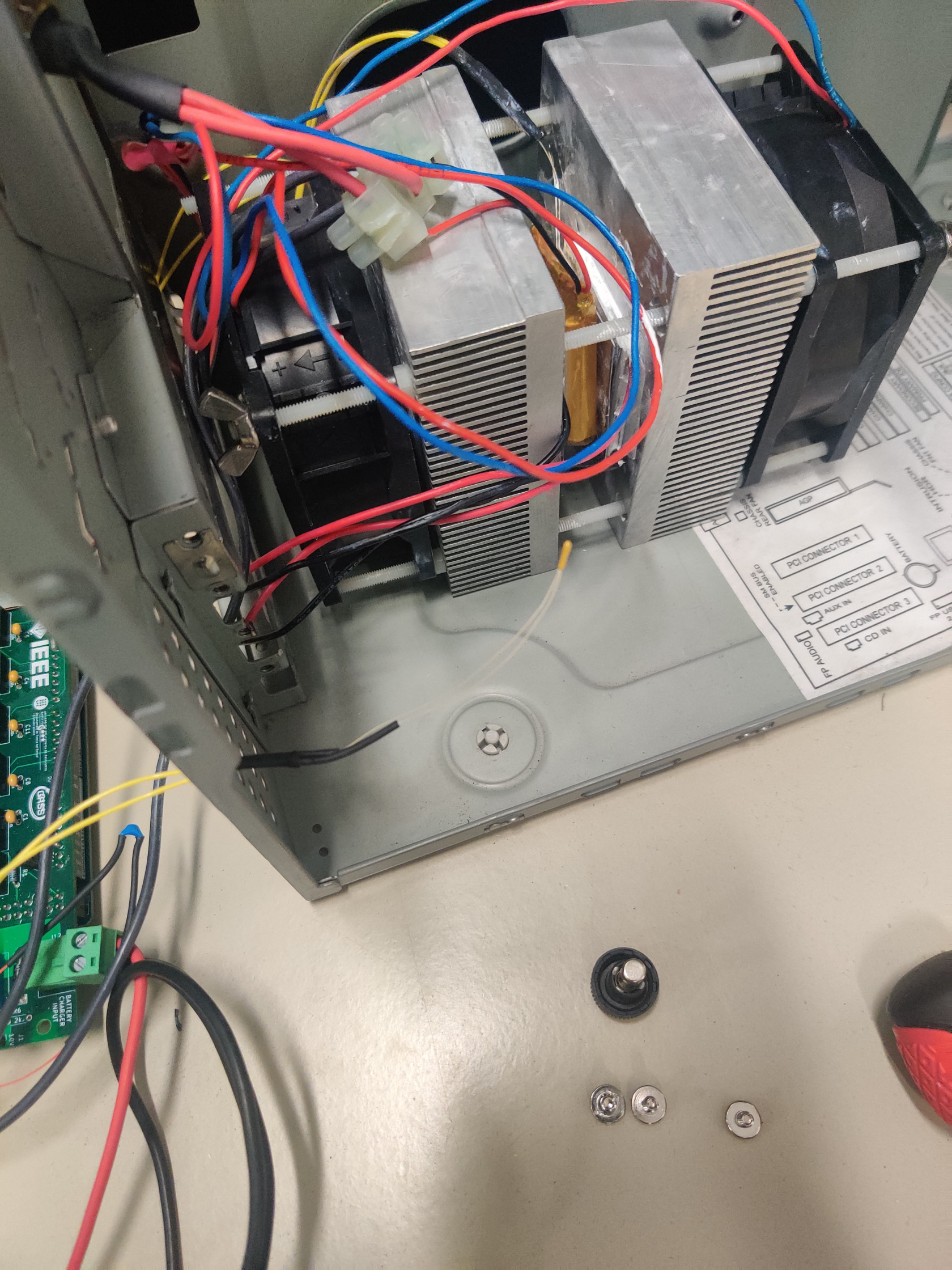](https://wiki.nanosatlab.space/uploads/images/gallery/2023-06/img-20230621-164651.jpg) 8. Close the metal box 9. Enable the 12V power supply output. 10. Connect the USB cable to the Arduino and PC and upload the charge .ino test code to the board. Select the adequate COM port on the Arduino IDE and remember it for the following steps. [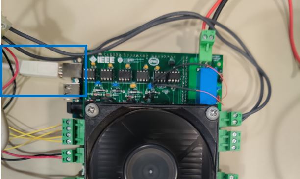](https://wiki.nanosatlab.space/uploads/images/gallery/2023-06/captura3.JPG) 11. Disconnect the USB cable from the PC. 12. Disable the 12V output. 13. Open PUTTY and select connection type: Serial and write down the Arduino COM port previously indentified. If the OS is Linux, it will probably be /dev/ttyACMX where 'X' is the port number. [](https://wiki.nanosatlab.space/uploads/images/gallery/2023-06/captura4.JPG) 14. In PUTTY go to the Logging tab and select Printable Output and select the folder where you want to save the test data. [](https://wiki.nanosatlab.space/uploads/images/gallery/2023-06/captura5.JPG) 15. Connect the battery cables to the terminal block labelled as BATERY respecting polarity and installing a Fuse of 2,5A between the battery test apparatus and the battery. [](https://wiki.nanosatlab.space/uploads/images/gallery/2023-06/captura6.JPG) 16. Enable both power supply channels. 17. Connect the USB cable to the PC and click on Open on the PUTTY software. 18. If all steps were performed correctly, the text START ARDUINO will be visible, and, after pressing any key of the keyboard, the test will start. Every 5 seconds a new line will be written indicating the voltage, current, accumulated power and temperature separated by a semicolon (“;”) 19. Each cycle end will be indicated on screen and at the beginning of each charge cycle the test iteration will be written. At the end of the entire test, a “TEST END” prompt will appear. Note that for a test of 10 iterations will take approximately 3 days to complete. 20. Disconnect USB cable. 21. Turn off power supplies. 19. After that the data will be available in the folder you selected before, and you can use the software you prefer to graph and analyse the result data from the CSV file. ## Test Results This battery degradation test has lasted 844 hours and taking into account that a full charge and discharge cycle lasts approximately 4 hours, a total of 211 full cycles have been performed. ## 1. Voltage [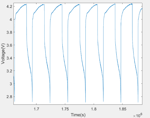](https://wiki.nanosatlab.space/uploads/images/gallery/2024-01/voltage.PNG) As it is seen, the votltage range is from 2.7 V to 4.3 V. It is faster for discharging than for charging because in charging mode when it is almost getting to the final charge voltage the cells are trying to get the equilibrium. For this reason, it is possible to see the slowest part from 4.1 V till 4.3 V. ## 2. Current [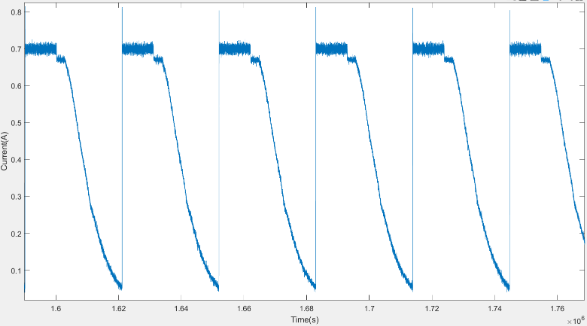](https://wiki.nanosatlab.space/uploads/images/gallery/2024-01/current.PNG) As the capacity of the battery is 1400 mAh, the current charge is 700 mA so as not to exceed the limit, for this reason we have a constant current and an almost linear discharge part as it discharges. The lowest current level is when it reaches to 2.7 V. ## 3. Energy [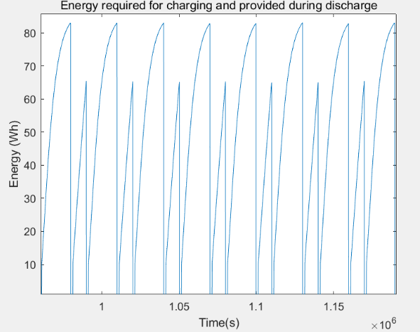](https://wiki.nanosatlab.space/uploads/images/gallery/2024-01/eenergy.PNG) In the previous graph, the highest plots are the energy in the charge cycle and the lowest ones represents the battery discharged or provided by the battery. It is seen that the last pic compared with the first one of the lowests plots is slightly lower than the first one. Let's see the complete charge and discharge cycles of the test: [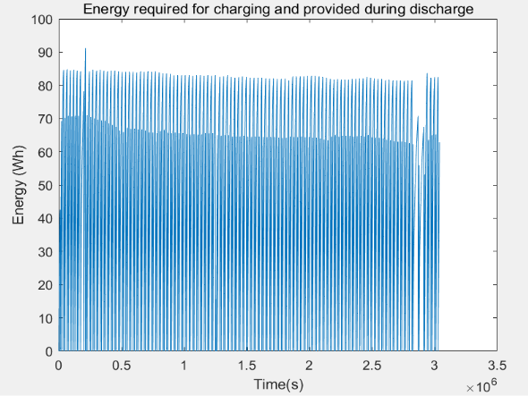](https://wiki.nanosatlab.space/uploads/images/gallery/2024-01/energy2.PNG) As the number of cycles increases, the battery capacity decreases. At the beggining of the test the battery provided around 70 Wh for one discharge cycle and at the end of the test it provided around 65 Wh for 1 discharge cycle. ## 4. Modules temperature [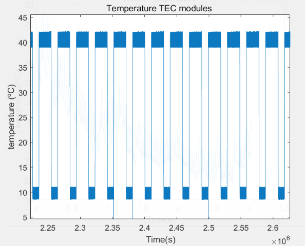](https://wiki.nanosatlab.space/uploads/images/gallery/2024-01/temperature-tec-modules.PNG) This plot represents the temperatures at the charge and discharge cycles. For charging the battery, the modules temperature is set to 40 ºC. For discharging, the temperature is set to 10 ºC. ## Conclusions It is seen in the energy plots the loss of effective energy provided by the battery. The battery starts providing 70 Wh for a discharge cycle and finally provides 65 Wh. This means that for every charge and discharge cycle is lost 23.7 mWh On the other hand, as it can be seen in the beginning of the voltage curves, the battery was subjected to a voltage higher than the maximum due to overheating of the power sources, and there were no serious consequences for it. Even though the test may not be entirely conclusive because of its time constraints, it does show the robustness of the battery. The PocketCube energy requirements are much smaller than the ones subjected in this test and therefore it can be concluded that the battery is suited for the mission. The code is available at: https://github.com/nanosatlab/pocat-sw/tree/main/Battery%20test%20aparatus/Arduino%20Code/Degradation_testing # Photodiodes Temperature CharacterizationThe main objective of this test is to characterise the temperature behaviour of the photodiode and calibrate its results.
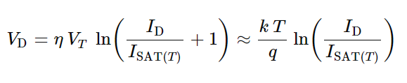
Following the Shockley Diode equation, the current coming out the photodiode depends of the temperature, following an exponential function.
The Shockley diode equation is the following one:
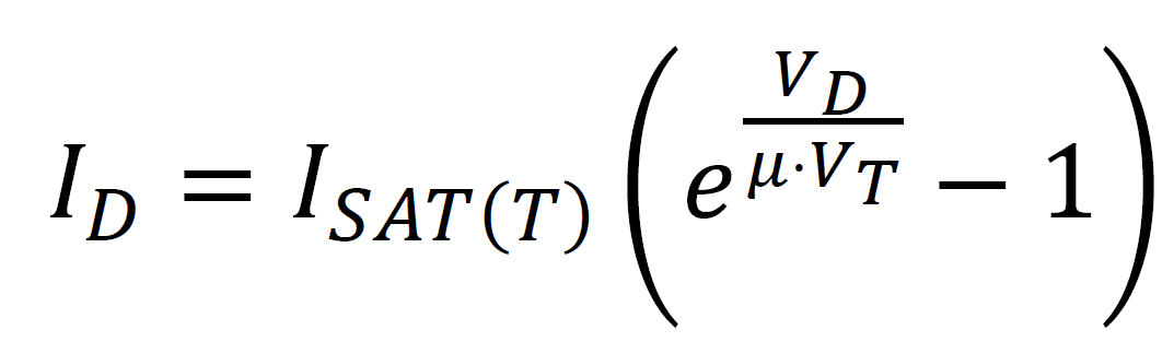
Where:
ID is the diode current.
Isat(T) is the reverse bias saturation current.
VD is the voltage of the diode.
VT is the thermal voltage.
μ is the idiality factor, it will be assumed that it is equal to 1.
In this equation there are two key parameters, the VT and the Isat(T) which are computed with the following formulas:
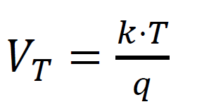
Where:
k is the Boltzman constant in [ j/k ].
T is the temperature of the diode in kelvins.
q is the elementary charge.
![]()
Where:
Tnom is the temperature in which the photodiode's characteristics are specified in the datasheet.
Eg is the energy gap.
Now the next step is to derive the sensitivity equation. To obtain it, you will have to derivate the Shockley diode equation in function of the temperature:

The sensitivity in function of the temperature will have this shape:
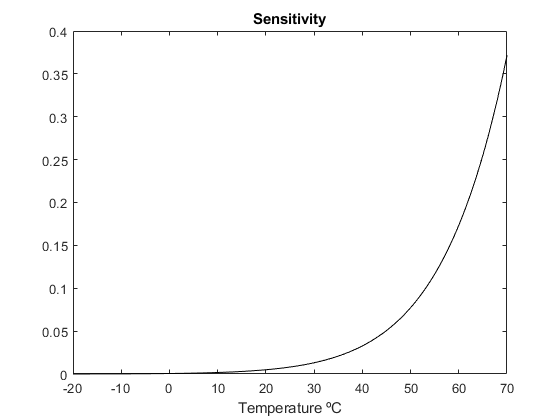
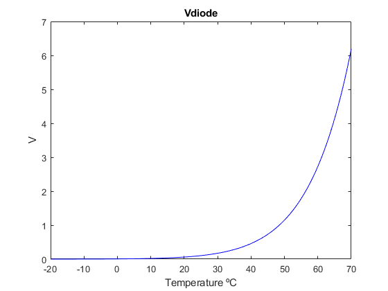
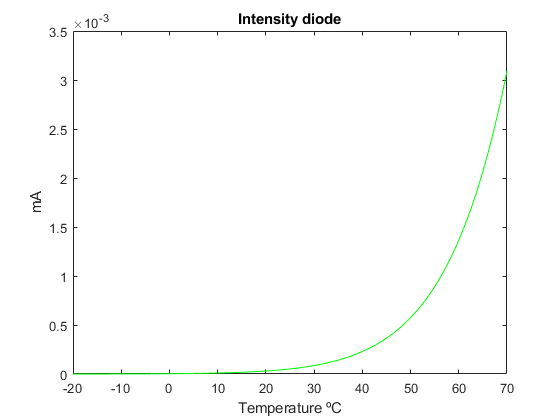
All the parameters that has been obtained are the following:
| Computed Isat(Tnom) | Measured voltage quantized values | Measured T |
At this part of the calibration the following steps have to be followed:

![]()
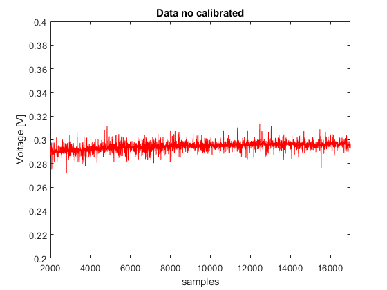
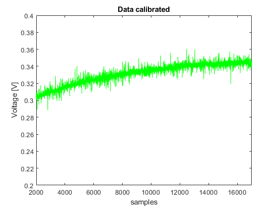
A simulation was conducted with a total of 17,000 samples of photodiode measurements taken at temperatures ranging from 15 to 35 degrees Celsius. As shown in the calibrated data, photodiode measurements increase with rising temperatures.
The calibration test has been conducted succesfully.
# Magnetorquer Polarisation verificationThe aim of this document is to clearly explain the procedure to verify the polarisation of the magnetorquers.
The aim of this test is to verify that the polarisation of the magnetorquers is the correct one.
| Requirement ID | Description |
|---|---|
| TST-MAGT-01 | The magnetorquers must generate a magnetic field direction in accordance with the left hand rule when current is being injected. |
The verification will be completed if the polarisation is the same as te theoretical computed using the right hand rule.


This test is designed to characterize and calibrate the ADCS gyroscopes, ensuring their precise performance under various conditions. The results will give us important information to improve the system that controls the satellite’s orientation, making the system more reliable and effective.
To conduct this test, an STM32L476RG Nucleo board is utilized as a simulator for the OBC-ADCS interface. Commands are sent to the Nucleo board, which subsequently requests data from the ADCS board.
To calibrate the gyroscope IIM 42652 we have done the following test:
First, the “Random walk phenomenon” of the gyroscope has to be characterized. The method will use the Allan’s variance. Once the samples of measurements has been taken, the standard deviation of the measurements will be plotted in function of the time. The results might be similar to the following ones:
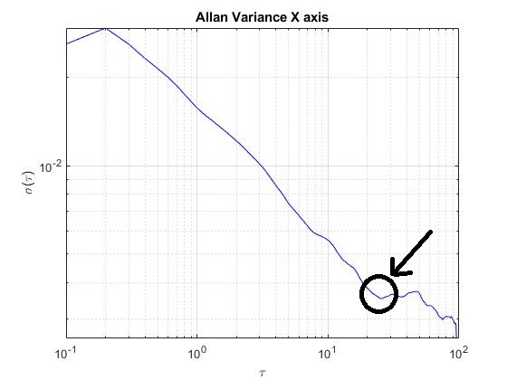


In these plots, it is observed the evolution of the standard deviation of the noise in the gyroscope samples. Approximately, in τ=10 s for the X and Z axis, and for τ=20 s, the standard variation tends to variate the slope of the line repeatedly, that happens because of the effect of the “Random walk phenomenon”.
Consequently, the gyroscope samples will be averaged for 10 seconds, using a sample frequency of 0.1 seconds. The total number samples that will be averaged is 100 samples.

The schematic used for the averaging algorithm is the following one:
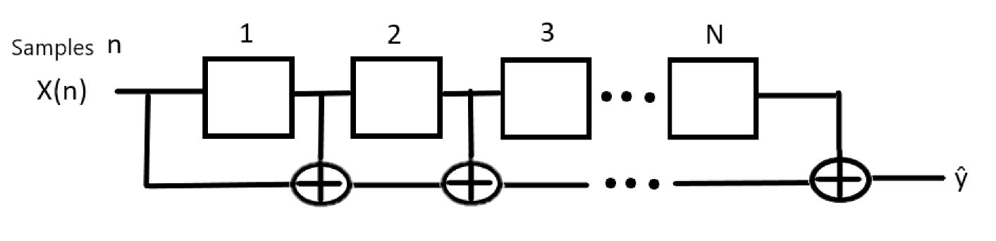
This algorithm functions as a circular queue that averages all the samples within it during each iteration, helping to reduce the effect of the "random walk phenomenon" in the gyroscope readings.
Afterwards, we will have to take at least 1000, or more, samples of data for each axi in differents situations using the algorithm of the previous section:
1- Static data measurements, all with a constant temperature.
2-Movement measurements
After that, in order to calibrate de measurements, the following formula will be used for each axis:
Data Calibrated = Data measured * sensitivity - Bias(Tº)
For each axis, plot the real data in function of the measured data using in the X axis the measured data and in the Y axis the real data. Afterwards, in the measured data vector use the static data and the constant velocity data, both obtained with the same temperature. Regarding the real data, also use the static real data and the real angular velocity data. Now you will have two figures, each one with different temperature, compute in both plots the line equation of the graphic and store the value of the slope coefficient of the equation.
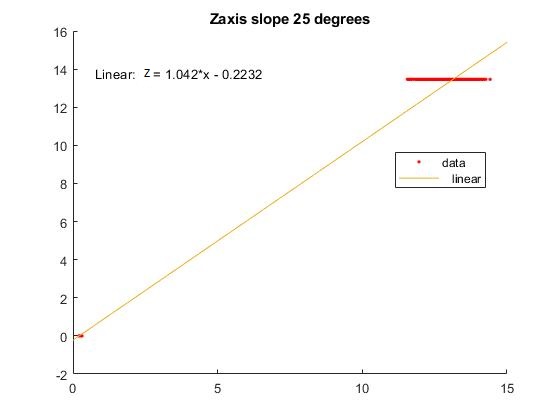
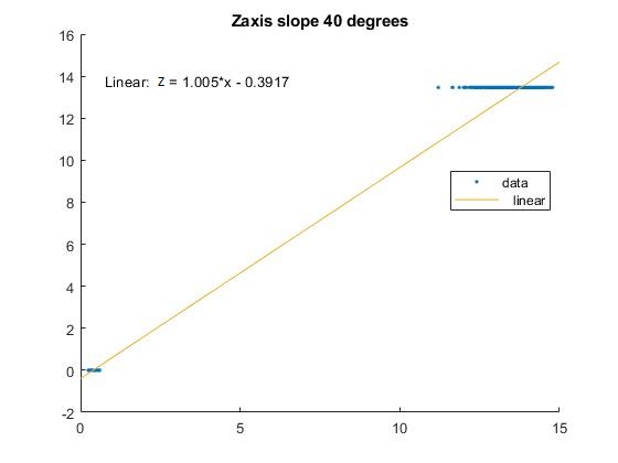
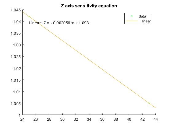
After obtaining the two slopes, one for the first temperature and the other for the second, the next step is to plot the slope, which is computed using the two previous calculated slopes, against the temperature and recalculate the line equation. This line equation will serve as the formula for calculating sensitivity as a function of temperature.
This procedure is repeated for each axis:
| Axis | Slope (25 ºC) | Slope (40 ºC) | Sensitivity equation |
| X | 1.073 | 1.085 | Xsens=-0.0009231*T(ºC)+1.05 |
| Y | 1.026 | 0.9912 | Ysens=-0.0029*T(ºC)+1.099 |
| Z | 1.042 | 1.005 | Zsens=0.002056*T(ºC)+1.093 |
For the next step of the calibration, the measured static data versus the temperature is plotted. This graphic will show us the evolution of the bias in respect to the temperature. Then, the equation of the line will be computed, which will be used in order to compute the Bias:
Bias( Tº) = m * Tº(temperature) + n
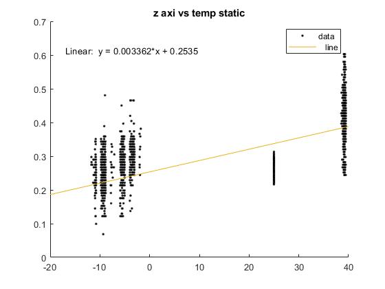
The results for each axis are:
| Axies | Bias equation |
| X | Bias=0.01388 * T(ºC)-0.1716 |
| Y | Bias=0.0005596 * T(ºC)-0.03862 |
| Z | Bias=0.003362 * T(ºC)+0.2535 |
The final calibrated data will be computed with the following equation:
Calibrated_data = Sensitivity(ºC) * Measured_data - Bias(ºC)
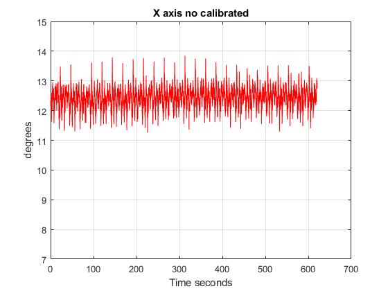
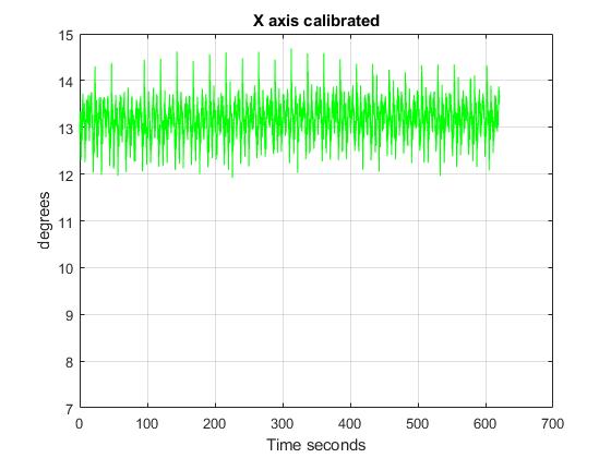
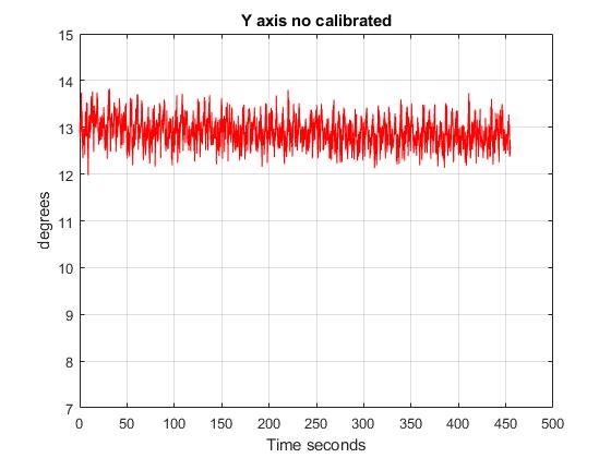
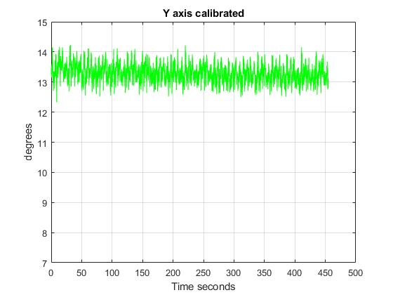
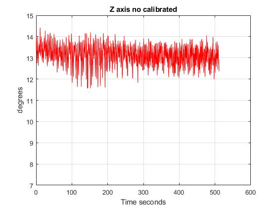
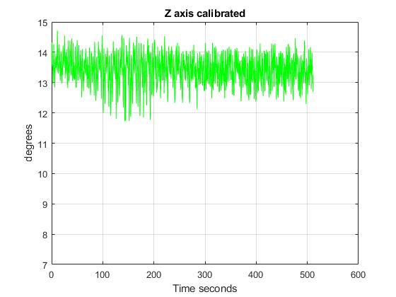
The test consisted of measurements of a real velocity of 13,6 degrees/s. The following plots show that the results of the calibration in all the axis.
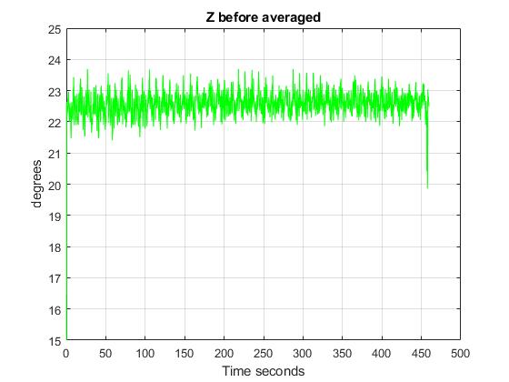
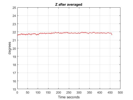
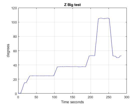
In addition, the following figures show the results of testing the averaged algorithm. The tests show how the gyroscope works once it has been calibrated. To do so, different velocities had been applied into the Z axis. Here are the results:
The temperature sensor inside the IIM 42652 could work wrongly if the chip has been exposed to high temperatures during the welding process. It is recommendable to check in the IIM 42652 documentation, which is the maximum temperature that the temperature sensor can withstand without getting damaged.
As all the requirements has been fulfilled, the test is completed.